← All notes

Reinforcement Learning for Large Language Models

July 30, 2026 · Updated September 26, 2026

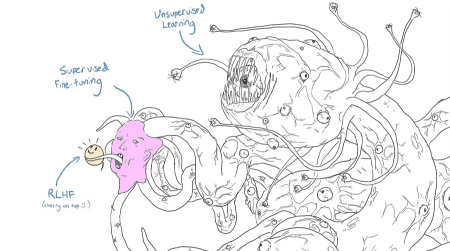
Yann LeCun has described intelligence with a cake analogy: “If intelligence is a cake, the bulk of the cake is unsupervised learning, the icing on the cake is supervised learning, and the cherry on the cake is reinforcement learning (RL).”

Following this, LLMs typically go through a three-step training pipeline:

1. Pre-training. Self-supervised learning on vast swaths of internet data makes up the majority of the cake, especially when viewed in compute spent (FLOPs).
2. Supervised fine-tuning (SFT). The beginning of post-training.
3. Reinforcement learning. Used for alignment, via RLHF (Reinforcement Learning from Human Feedback), and for creating “reasoning” or “thinking” models, via RLVR (Reinforcement Learning with Verifiable Rewards).

Reinforcement Learning from Human Feedback (RLHF)

RLHF is the original alignment method. Its goal is to align LLMs with human preferences.

There is no verifiable answer to check against for most of what we ask a model to do, so RLHF gets its signal from people instead. Thousands of human judgements are collected, each one a pairwise preference between two candidate answers to the same prompt: A over B, D over C, and so on. A neural network, the reward model, is then trained to imitate those preferences, so it can score responses the way the annotators would have.

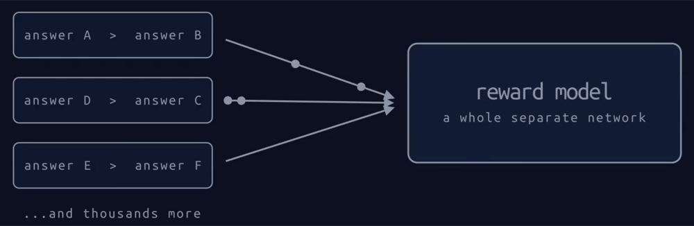
That reward model is what the policy is then optimized against, which is the proxy the RLVR section below contrasts with.

It is worth being precise about what this buys. RLHF makes a model safer with respect to the behaviors and situations that its training and evaluation data represent. It does not guarantee safety under distribution shift. A prompt unlike anything the annotators considered can still pull out the behavior the training was meant to suppress, which is the point the painted-on face above is making.

TODO: will update this section later.

RL Formulation for LLMs

Applying any of this to an LLM starts with fixing what each piece of the RL vocabulary refers to once the environment is a model emitting tokens.

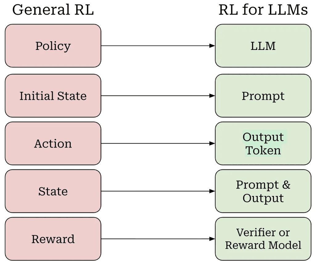
There is no transition function to speak of in this setup, because the transition is completely deterministic. Starting from a prompt $x$, our initial state is $s_0 = \{x\}$. Once the LLM predicts a token $t_1$ we are in $s_1 = \{x, t_1\}$, and once it predicts $t_2$ we are in $s_2 = \{x, t_1, t_2\}$: the subscript is the timestep, counting how many tokens have been generated so far.¹ In other words, our state is just the running completion being generated by the LLM for a given prompt $x$.

For LLMs, there are two key ways in which RL can be formulated, differing in how they model actions:

• Bandit formulation: the entire completion or response from the LLM is modeled as a single action.
• Markov decision process (MDP) formulation: each token within the LLM’s output is modeled as an individual action.

In the context of LLMs, we already know how to compute the probability of both individual tokens and the full completion for a prompt. Therefore, we have the ability to model RL using either an MDP or a bandit formulation.² Given that LLMs usually only receive outcome rewards, however, the bandit formulation, despite being very simple, is quite fitting for LLMs. REINFORCE and RLOO adopt the bandit formulation, while algorithms like PPO use a per-token MDP formulation.³

Policy Gradients for LLMs

Before PPO, the plainest thing that can be done with this setup is the policy gradient itself. Its estimator, derived here, is

We are increasing the probability of actions taken on trajectories with high rewards: taking a step with this gradient pushes up the log-probability of each action in proportion to $r(\tau)$, the sum of all the rewards obtained along that trajectory.

Reading it back through the mapping above: a trajectory $\tau_i$ is one completion, the inner sum runs over that completion’s tokens, and $r(\tau_i)$ is the single outcome reward a verifier or reward model returns once the completion is finished. Under the bandit formulation the whole inner sum collapses into the log-probability of the completion as a single action; under the per-token MDP formulation it stays a sum over tokens.

In code, one training step of the basic policy gradient is⁴:

REINFORCE & RLOO for LLMs

Adapted from Cameron R. Wolfe, “REINFORCE: Easy Online RL for LLMs”.

REINFORCE

The structure of the policy gradient used by REINFORCE is similar to the baselined policy gradient estimate covered earlier. However, REINFORCE specifically uses the average of rewards observed during RL training as a baseline. This average can be computed in a few different ways; e.g., a moving average of rewards throughout training or an average of rewards present in the current batch.

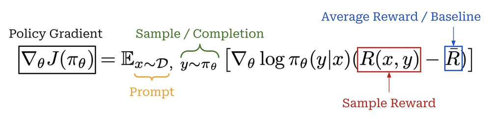
The figure follows the source’s notation: the completion is $y$ and its reward $R(x, y)$, written as the action $a$ and reward $r$ elsewhere in this note.

The expression for the policy gradient in REINFORCE is shown above. To compute a gradient update over a batch, we perform the following steps:

1. Generate a completion for each prompt using the current policy.
2. Store the log probabilities for the tokens in each completion.
3. Assign a reward to each completion (usually with a reward model).
4. Obtain a baseline by taking an average of rewards.
5. Compute the advantage by subtracting the baseline from the reward.
6. Compute the sum of log probabilities multiplied by the advantage for each completion, then average over the batch to form a Monte Carlo estimate.

Note that this is a bandit formulation: the advantage here is defined at the completion level, rather than separately for every token as in the per-token MDP view.⁵

We also incorporate the Kullback-Leibler (KL) divergence with respect to a reference policy, usually a prior SFT-trained checkpoint of our model, into REINFORCE. Adding the KL divergence into RL regularizes the training process and allows us to ensure that our policy does not deviate significantly from the reference policy. There are several different approaches for approximating KL divergence. A common approach is to approximate it as the difference in log probabilities between the policy and the reference policy.⁶ Once we have made this approximation, the KL divergence is directly incorporated into the reward:

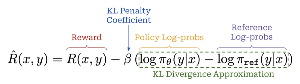
Note that unlike PPO and GRPO, the KL divergence here is not incorporated into the loss function, but directly into the reward.

Most LLMs are trained using an outcome reward setting, meaning that only the final <eos> token generated by the LLM is assigned a reward. The KL divergence, however, is computed on a per-token basis, and is subtracted from the reward as above. This is where the choice of formulation starts to matter: REINFORCE treats the entire completion as a single action, whereas regular PPO treats each completion token as an individual action. Since typically only the <eos> token gets a true reward, which is very sparse, PPO (which is formulated as an MDP) would attribute that reward to the <eos> token alone, whereas REINFORCE attributes it to the whole completion.

We create a completion-level (bandit formulation) reward by summing the per-token KL divergences and rewards over the sequence. Similarly, we can sum the token-level log probabilities to get the log probability of the completion (or trajectory). We can then use these completion-level components to compute the policy gradient much as before:

1. Subtract the baseline (average reward) from the completion-level reward.
2. Multiply this difference by the completion log probability.
3. Run a backward pass to compute the final policy gradient.

The figure below runs the whole process on an example completion, with numbers at every step.

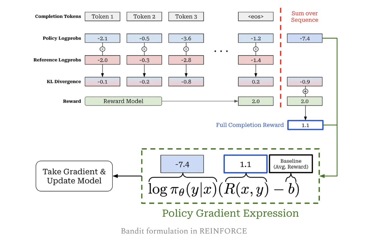
This computes the policy gradient for a single prompt and completion pair, and we generally average that gradient over a batch of completions.

REINFORCE Leave One Out (RLOO)

In REINFORCE, we generate a single on-policy completion per prompt during training and use the rewards from these completions to form our baseline via a moving average or an average of rewards in the batch.⁷

The problem with this is that an average reward taken across completely different prompts isn’t necessarily very meaningful. Different prompts can have very different reward distributions, and ideally we’d like to ask whether a given completion is good compared with other completions for the same prompt. This is what REINFORCE leave-one-out (RLOO) does. Specifically, it:

1. Samples multiple ($K$) completions per prompt.
2. Uses those completions to compute the reward average separately for each individual prompt.

Given $K$ completions $\{y_1, y_2, \ldots, y_K\}$ for the same prompt $x$, RLOO defines the baseline for completion $y_i$ as shown below, which is simply an average over all rewards for completions to prompt $x$ excluding the completion itself, $y_i$. We “leave out” the reward of the completion for which the policy gradient is being computed and average over the rewards of the other completions to the same prompt. The reason is that when evaluating $y_i$, we want the baseline to be constructed from independent alternative samples, rather than allowing $y_i$‘s own reward to influence the baseline it is measured against. Hence: leave one out.

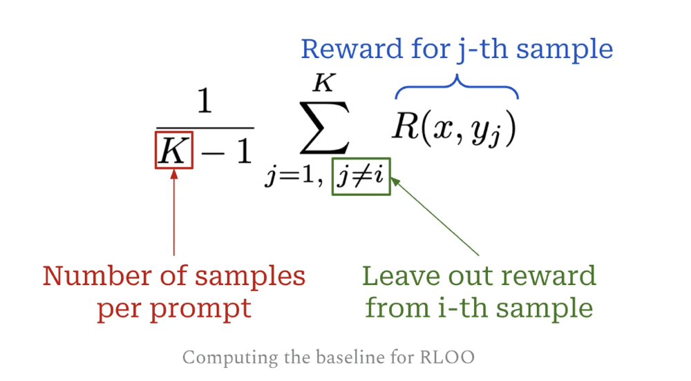
From here, we can compute the advantage estimate in RLOO by (i) computing this baseline for every completion for the prompt and (ii) subtracting the baseline from the reward received by that completion, as in the first equation below.⁸

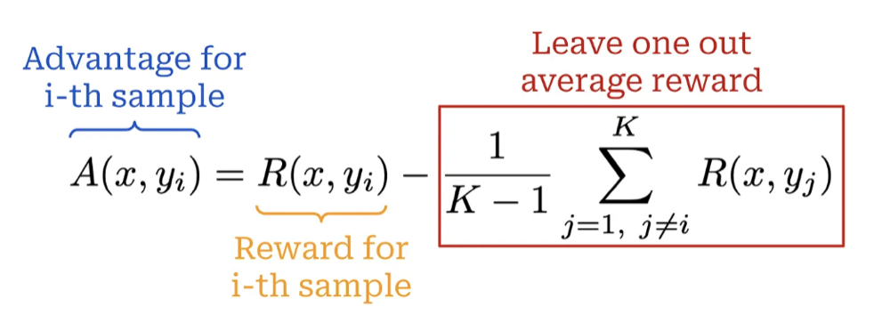
To compute the baseline efficiently, we can first compute a fixed average reward over the $K$ completions and reformulate the advantage as in the second equation below. This lets us compute the average reward once and avoid re-computing the leave-one-out average for all $K$ completions to the prompt $x$.

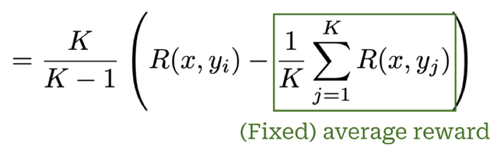
This modified advantage estimate can be plugged into the same policy gradient expression used by REINFORCE. As in REINFORCE, RLOO uses a per-completion (as opposed to per-token) loss, and there is no learned value model.

For each completion we have its advantage $A_i$ and its log probability $\log \pi_\theta(y_i \mid x_i)$. Writing $B$ for the number of prompts in the batch and $K$ for the number of completions sampled per prompt, the loss is

from which we take $\nabla_\theta L$ and a single optimizer step:

So a batch of 32 prompts with $K = 8$ completions each puts $32 \times 8 = 256$ completion samples behind one gradient step. The leave-one-out baseline lowers variance relative to standard REINFORCE by using multiple samples per prompt to derive the policy gradient estimate. Compared to a single-sample approach, this benefits training stability, speed, and performance.

KL Divergence for LLMs

The definition, its discrete and continuous forms, and why it is not symmetric are in the standalone KL divergence note. This section is about what it is doing once the two distributions are language models.

Throughout LLM post-training, there are many cases where we optimize our model subject to a KL divergence constraint. The canonical optimization objective used within RLHF has the form shown below.

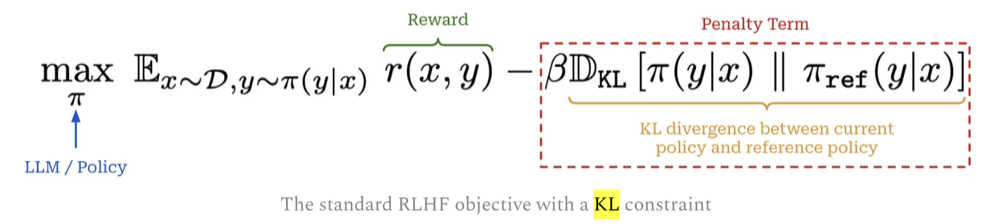
As we can see, we want to maximize rewards while minimizing a penalty term, the KL divergence weighted by $\beta$, that is subtracted from these rewards. A larger $\beta$ puts more weight on staying close to the reference policy. A smaller $\beta$ allows more change in pursuit of reward. We usually estimate the KL divergence between the completion distributions predicted by our current policy and a fixed reference policy, often the original SFT model. Intuitively, adding this constraint to the reward used during RL training, as shown above, discourages the policy being trained from drifting too far from the reference policy. For a prompt $x$, this KL divergence has the following form:

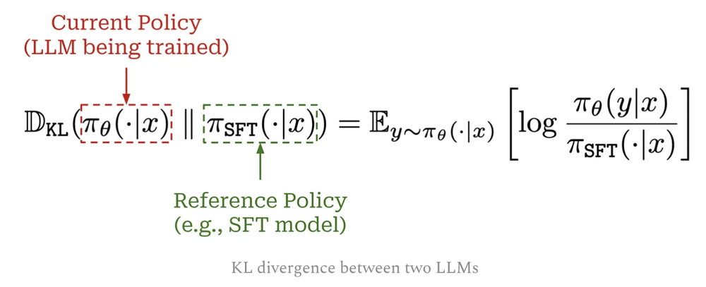
This form of the KL divergence looks at the ratio of probabilities predicted by both the current and reference model for a completion $y$ given a prompt $x$ as input. The probability of a completion $y$ is simply the product of next token probabilities predicted by the LLM for each token within a completion. By computing the KL divergence over these completion probabilities, we capture the similarity between the token distributions predicted by the two models.⁹

The log ratio for a sampled completion is exact for that particular completion. KL, however, compares two entire completion distributions, so its exact definition includes every possible completion:

This is the conditional KL for one prompt. During training, we typically average this quantity over prompts drawn from a prompt distribution $\mathcal{D}$.

We don’t compute KL exactly and instead estimate it because of the large number of possible completions. Even with a vocabulary of only 100 tokens and completions that are exactly 10 tokens long, there are

possible completions. Computing and adding one term for each is impractical. Another practical reason is that during training we generally do not retain the full distribution (all token probabilities) at every position. To save GPU memory and I/O, we keep only the log-probabilities of the tokens actually generated along each trajectory.

From the exact KL to a sampled token. At each generated prefix, let

denote the prompt together with the tokens generated before position $t$. The exact reverse KL between the current and reference next-token distributions is

Computing this expression directly requires summing over the entire vocabulary at every generated position. A rollout instead supplies one token sampled from the current policy,

Evaluating that token under both policies gives the one-sample estimator

Conditioned on the prefix, this estimator is unbiased:

This is ordinary Monte Carlo estimation with one sample, providing a KL signal at every generated token. An individual sampled value can be negative even though the exact KL is nonnegative.

Summing these sampled token-level log ratios gives the log ratio for the complete sampled completion:¹⁰

A good estimator should ideally be unbiased, so it has the right mean, and low-variance, so a finite batch gives a stable answer. For each sampled prompt-completion pair, define the inverse likelihood ratio

Three common choices are

For samples from the current policy, $k_1$ is unbiased but can have high variance. $k_2$ can reduce variance when the two policies are close, but it is biased. $k_3$ is unbiased, nonnegative, and typically lower-variance. The standard PPO-style log-ratio penalty described above uses $k_1$, while the original DeepSeekMath formulation of GRPO uses $k_3$ at each token. Implementations can vary; see John Schulman’s note on KL approximation for the derivations.

Whichever estimator we choose, the computation follows the same pattern:

1. Sample. Draw $N$ prompt-completion pairs, with $x^{(i)} \sim \mathcal{D}$ and $y^{(i)} \sim \pi_\theta(\cdot \mid x^{(i)})$.
2. Compute log-probabilities. Evaluate each completion under both models to obtain $\log \pi_\theta(y^{(i)} \mid x^{(i)})$ and $\log \pi_{\mathrm{ref}}(y^{(i)} \mid x^{(i)})$, then form $\log w_i = \log \pi_{\mathrm{ref}} - \log \pi_\theta$.
3. Apply the estimator. Compute $k_1(w_i)$, $k_2(w_i)$, or $k_3(w_i)$ for each pair.
4. Average. Average those values over the batch.

Using $k_1$ gives the estimator already developed above:

Each bracketed log ratio is exact for its sampled prompt-completion pair, but their finite average is a Monte Carlo estimate of the KL averaged over the prompt distribution. As $N$ grows, this empirical average approaches the true prompt-averaged KL divergence.¹¹

In PPO, the token-level penalty and the batch-level Monte Carlo estimate use the same samples. With $k_1$, each completion’s log ratio is the sum of its sampled token log ratios. PPO can apply those sampled per-token log ratios directly to the corresponding token rewards, while summing them within each completion and averaging across the batch gives the scalar KL estimate used for monitoring or adapting $\beta$.

Proximal Policy Optimization (PPO) for LLMs

PPO is what the RLHF pipeline above optimizes with, and relies upon the MDP formulation. The derivation, from the importance ratio through clipping to the surrogate objective, is in the actor-critic note; this section is about what the algorithm looks like in the setup above.

In the context of LLMs, during generation actions are taken by selecting a token from the model’s next-token distribution: each token is its own action. After a token is predicted, it is added to the current state and used by the LLM to predict the next token. Eventually, the LLM predicts a stop token (e.g. <|end_of_text|> or <eos>) to complete the generation process, thus yielding a complete trajectory.

As we saw in the REINFORCE section, we first sample a batch of prompts and generate completions to these prompts with our LLM or policy. Then, we compute the rewards for these completions and use these rewards to derive a policy update.

Each training iteration of PPO performs the following sequence of steps:

1. Sample a diverse batch of prompts.
2. Generate a completion from the policy for each prompt.
3. Compute advantage estimates for each completion.
4. Perform several policy updates over this sampled data.

To see the whole thing in one place, here is a single token’s PPO update worked end to end, for an LLM answering “What’s 2 + 2?”:

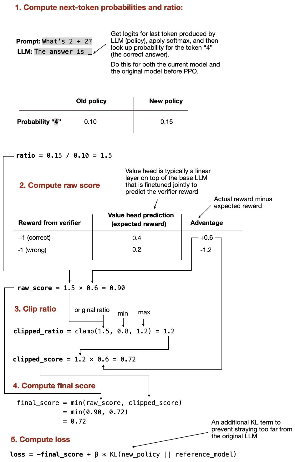
ratio         = new_policy_prob / old_policy_prob
raw_score     = ratio * advantage
advantage     = actual_reward - expected_reward
clipped_ratio = clamp(ratio, 0.8, 1.2)
clipped_score = clipped_ratio * advantage
final_score   = min(raw_score, clipped_score)
loss          = -final_score
              + β * KL(new_policy || reference_policy)

The value head reads the same text the policy did, What's 2 + 2? The answer is, and predicts the reward the verifier will end up handing back. Subtracting that prediction from the reward actually received is what turns a raw reward into the advantage in step 2.

The last line adds one piece the derivation elsewhere doesn’t cover. LLM setups usually attach a KL penalty to the clipped objective, weighted by $\beta$, and it’s measured against a reference model: the model as it was before RL started, frozen for the entire run. That’s a different thing from the snapshot in the ratio’s denominator, which is refreshed every batch. The ratio keeps a single update from moving too far; the KL term keeps the whole run from drifting far from where it began.

PPO’s inner loop takes several gradient steps on one collected batch, and what sits in the ratio’s denominator through all of them is worth being precise about. $\pi_{\theta_{\text{old}}}$ is not the model from the previous gradient step; it’s a frozen snapshot taken before the batch was collected. Nothing trains that copy, and it does two jobs at once: it generates the rollouts (prompt 1 → response A, prompt 2 → response B, and so on), and it supplies $\pi_{\theta_{\text{old}}}(a \mid s)$ for every ratio computed off them. So as the inner loop runs, the numerator $\pi_\theta$ moves every step, after one update, then after two, then after three, while the denominator stays $\pi_{\theta_{\text{old}}}$ the whole way through. The advantage is frozen alongside it: $\hat{A}$ is computed once from this batch and reused unchanged by every step, recomputed once per rollout rather than once per optimizer step.

For LLM RL, “several steps” usually means 2 to 10 epochs over the same batch. Then the data is discarded, $\theta_{\text{old}} \leftarrow \theta$ makes the latest model the new frozen snapshot (playing both roles again), and the loop restarts from a completely fresh batch. Resetting that often is what bounds the staleness that several gradient steps on one batch introduce: every action and reward in the batch came from $\pi_{\theta_{\text{old}}}$, so still training on them twenty updates later means optimizing against behavior the model no longer exhibits.

The reason to squeeze several steps out of one batch at all is cost. Generating rollouts dominates: a single batch might mean generating 16,000 completions, scoring each one with a reward model or verifier, and computing advantages, which can take minutes. A gradient step on data already sitting in GPU memory is cheap by comparison, so taking exactly one update per batch would mean paying the expensive part over and over for one cheap step each time. Despite the importance ratio, PPO is still usually called an on-policy algorithm, because the data it trains on always comes from the current policy or one that’s only a few optimization steps old.

KL Divergence for PPO: There are two common ways to incorporate KL divergence into PPO training. The first is to subtract it from the reward, as in the KL-adjusted reward shown earlier. The second is to add it directly as a penalty term in the training objective, as in the RLHF objective with a KL constraint. In both cases, the aim is to maximize reward without allowing the current policy to drift too far from the reference policy.

Both approaches have been used successfully and represent two views of essentially the same regularized objective. Papers commonly write KL divergence as a penalty in the objective, while PPO implementations often incorporate its sampled token-level contribution into the reward because this integrates naturally with return and advantage computation.

For the reward-penalty implementation, a typical PPO rollout proceeds as follows:

1. Sample a batch of prompts.
2. Freeze a snapshot of the current policy as $\pi_{\theta_{\text{old}}}$ and use it to generate completions for those prompts.
3. For every generated token, record the log-probability assigned to that token by both $\pi_{\theta_{\text{old}}}$ and the frozen reference policy $\pi_{\mathrm{ref}}$, usually the original SFT model $\pi_{\mathrm{SFT}}$. Computing the exact categorical KL at each position would instead require both models’ full probability distributions over the vocabulary.
4. Compute a sampled per-token KL term from the log ratio $\log \pi_{\theta_{\text{old}}}(a_t \mid s_t) - \log \pi_{\mathrm{ref}}(a_t \mid s_t)$, or use another KL estimator.
5. Multiply each token’s KL term by $\beta$ and subtract it from that token’s reward. In the alternative formulation, add the corresponding penalty directly to the training loss.
6. Aggregate the token-level terms for monitoring, commonly by summing over each completion and averaging across the batch.¹²

The reference policy remains fixed throughout PPO training, so it serves as a stable anchor for the behavior learned during SFT. A low $\beta$ creates a weak penalty, giving the current policy more freedom to pursue reward but increasing the risk of excessive drift. A high $\beta$ creates a strong penalty, preserving behavior closer to the reference policy but potentially limiting reward improvement.

Choosing $\beta$ often requires experimentation. An adaptive KL controller can adjust it using the KL observed in each batch: when KL exceeds a target, the controller increases $\beta$ to strengthen the constraint; when KL falls below the target, it decreases $\beta$ to permit more optimization. See ApX’s “The Role of the KL Divergence Penalty” for a broader overview.

Advantage in PPO: The advantage function is defined as the difference between the state-action value function and the value function, $A(s_t, a_t) = Q(s_t, a_t) - V(s_t)$. In PPO, we estimate the state-action value function using the actual reward observed for a trajectory. The value function, in contrast, is estimated using a learned model, the critic. For an LLM completion with $T$ generated tokens, PPO evaluates this quantity at every token-level state-action pair, producing $[\hat{A}_1, \hat{A}_2, \ldots, \hat{A}_T]$: each token position receives its own advantage value.¹³

The critic that supplies $V(s_t)$ is usually built by copying the policy and swapping its language modeling head, which outputs one logit per vocabulary token, for a value head: a small linear layer that maps each position’s hidden state to a single scalar. That copy is initialized from the policy’s weights, but it trains on its own objective from then on, so the two networks drift apart as PPO proceeds.

Taking a partial response as input, the critic predicts the expected final reward for every token position in the sequence. Most LLMs are trained with outcome supervision, meaning a reward is only assigned once the model has generated a complete response, after the <eos> token has been emitted. The critic and the reward model are similar in that both are learned models that predict rewards. The difference is what each one is given: the critic predicts an expected reward from a partial completion, while the reward model scores an entire finished response.

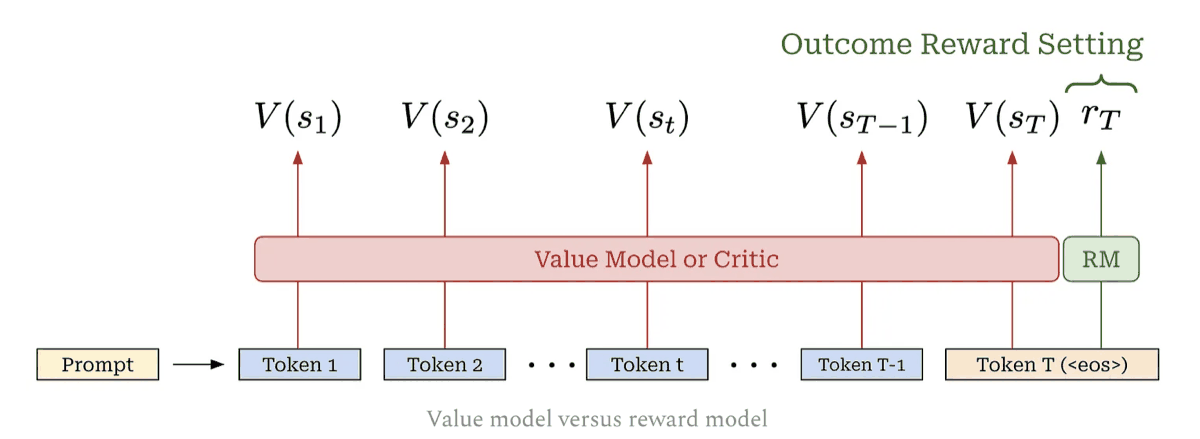
The value function is on-policy. Unlike the reward model, which is fixed at the start of RL training, the critic is trained alongside the LLM at every policy update so its predictions stay on-policy. This is done by adding an extra mean-squared error (MSE) loss, as in training the value network, to the surrogate loss.

The update in code

Here is the whole thing as code, in two files. ppo.py holds the algorithm: it caches the rollout targets once, then takes several gradient steps against that frozen snapshot. ppo_llm_example.py is the harness around it, wiring up a small pretrained model, a frozen reference copy, and a critic with a value head, then running one update on a batch of three prompts. That batch is small enough to follow by hand, so it is worth walking the tensors through ppo_update once: every shape, every mask, and the numbers that come out at each step are traced in a footnote.¹⁴

import torch
import torch.nn.functional as F


def token_log_probs(model, input_ids, attention_mask):
    # Position t predicts token t + 1.
    logits = model(
        input_ids=input_ids,
        attention_mask=attention_mask,
    ).logits[:, :-1]

    logps = F.log_softmax(logits.float(), dim=-1)

    return logps.gather(
        dim=-1,
        index=input_ids[:, 1:].unsqueeze(-1),
    ).squeeze(-1)


def critic_values(critic, input_ids, attention_mask):
    # Assumes CRITIC returns [B, L] or [B, L, 1].
    values = critic(
        input_ids=input_ids,
        attention_mask=attention_mask,
    )

    if values.ndim == 3:
        values = values.squeeze(-1)

    # Value before each target token is generated.
    return values[:, :-1].float()


def response_mean(x, mask):
    # Equal weight per response.
    x = x.masked_fill(~mask, 0.0)
    return (
        x.sum(dim=-1)
        / mask.sum(dim=-1).clamp_min(1)
    ).mean()


def ppo_update(
    LLM,
    REF,
    CRITIC,
    optimizer,
    completions,       # [B, L]: prompt + response + padding
    attention_mask,    # [B, L]: valid prompt and response positions
    completion_mask,   # [B, L - 1]: response target positions only
    outcome_rewards,   # [B]: frozen reward-model scores
    num_ppo_steps=4,
    kl_beta=0.1,
    critic_weight=0.5,
    ppo_eps=0.2,
    gamma=1.0,
    max_grad_norm=1.0,
):
    mask = completion_mask.bool()

    if mask.shape != completions[:, 1:].shape:
        raise ValueError("completion_mask must have shape [B, L - 1].")

    if not mask.any(dim=-1).all().item():
        raise ValueError("Every example must contain a response token.")

    # Disable dropout. eval() still allows gradients.
    LLM.eval()
    REF.eval()
    CRITIC.eval()

    # LLM must still be the policy that generated this rollout.
    # Cache all rollout targets BEFORE any optimizer updates.
    with torch.no_grad():
        old_token_logps = token_log_probs(
            LLM, completions, attention_mask
        )
        ref_token_logps = token_log_probs(
            REF, completions, attention_mask
        )
        old_values = critic_values(
            CRITIC, completions, attention_mask
        )

        # Fixed KL-shaped rollout rewards.
        sampled_kl = old_token_logps - ref_token_logps
        token_rewards = (-kl_beta * sampled_kl).masked_fill(
            ~mask, 0.0
        )

        # Actual final response position, including the prompt offset.
        positions = torch.arange(
            mask.size(1), device=mask.device
        ).unsqueeze(0).expand_as(mask)

        last_indices = positions.masked_fill(
            ~mask, -1
        ).amax(dim=-1)

        rows = torch.arange(mask.size(0), device=mask.device)

        token_rewards[rows, last_indices] += outcome_rewards.to(
            device=token_rewards.device,
            dtype=token_rewards.dtype,
        )

        # Monte Carlo return-to-go.
        # Assumes contiguous responses and terminal episode endings.
        returns = torch.zeros_like(token_rewards)
        running_return = torch.zeros_like(token_rewards[:, 0])

        for t in reversed(range(token_rewards.size(1))):
            running_return = (
                token_rewards[:, t] + gamma * running_return
            )
            running_return = running_return.masked_fill(
                ~mask[:, t], 0.0
            )
            returns[:, t] = running_return

        # Fixed advantages: do NOT recompute after critic updates.
        advantages = (returns - old_values).masked_fill(
            ~mask, 0.0
        )

    trainable_params = [
        parameter
        for group in optimizer.param_groups
        for parameter in group["params"]
        if parameter.requires_grad
    ]

    metrics = []

    # Reuse this rollout for multiple full-batch gradient steps.
    for step in range(num_ppo_steps):
        token_logps = token_log_probs(
            LLM, completions, attention_mask
        )
        values = critic_values(
            CRITIC, completions, attention_mask
        )

        log_ratio = (token_logps - old_token_logps).masked_fill(
            ~mask, 0.0
        )
        ratio = log_ratio.exp()

        clipped_ratio = ratio.clamp(
            1.0 - ppo_eps,
            1.0 + ppo_eps,
        )

        actor_loss = -response_mean(
            torch.minimum(
                ratio * advantages,
                clipped_ratio * advantages,
            ),
            mask,
        )

        critic_loss = response_mean(
            (values - returns).square(),
            mask,
        )

        loss = actor_loss + critic_weight * critic_loss

        optimizer.zero_grad(set_to_none=True)
        loss.backward()

        torch.nn.utils.clip_grad_norm_(
            trainable_params, max_grad_norm
        )

        optimizer.step()

        metrics.append({
            "step": step + 1,
            "loss": loss.detach().item(),
            "actor_loss": actor_loss.detach().item(),
            "critic_loss": critic_loss.detach().item(),
        })

    return metrics

"""Run the PPO update on a batch using a pretrained causal language model."""

from copy import deepcopy

import torch
import torch.nn as nn
from transformers import AutoModel, AutoModelForCausalLM, AutoTokenizer

from ppo import ppo_update


MODEL_NAME = "sshleifer/tiny-gpt2"


class TransformerCritic(nn.Module):
    """A pretrained transformer backbone with a token-level value head."""

    def __init__(self, model_name):
        super().__init__()
        self.backbone = AutoModel.from_pretrained(
            model_name,
            local_files_only=True,
        )
        self.value_head = nn.Linear(
            self.backbone.config.hidden_size,
            1,
        )

    def forward(self, input_ids, attention_mask):
        hidden_states = self.backbone(
            input_ids=input_ids,
            attention_mask=attention_mask,
        ).last_hidden_state
        return self.value_head(hidden_states).squeeze(-1)


def make_completion_batch(tokenizer, prompts, responses):
    """Tokenize prompt/response pairs and mark response target positions."""
    sequences = []
    prompt_lengths = []

    for prompt, response in zip(prompts, responses, strict=True):
        prompt_ids = tokenizer.encode(prompt, add_special_tokens=False)
        response_ids = tokenizer.encode(response, add_special_tokens=False)
        sequences.append(
            prompt_ids + response_ids + [tokenizer.eos_token_id]
        )
        prompt_lengths.append(len(prompt_ids))

    max_length = max(map(len, sequences))
    batch_size = len(sequences)
    completions = torch.full(
        (batch_size, max_length),
        tokenizer.pad_token_id,
        dtype=torch.long,
    )
    attention_mask = torch.zeros(
        (batch_size, max_length),
        dtype=torch.long,
    )
    completion_mask = torch.zeros(
        (batch_size, max_length - 1),
        dtype=torch.bool,
    )

    for row, (sequence, prompt_length) in enumerate(
        zip(sequences, prompt_lengths, strict=True)
    ):
        sequence_length = len(sequence)
        completions[row, :sequence_length] = torch.tensor(sequence)
        attention_mask[row, :sequence_length] = 1

        # Shifted index prompt_length - 1 predicts the first response token.
        completion_mask[
            row,
            prompt_length - 1 : sequence_length - 1,
        ] = True

    return completions, attention_mask, completion_mask


def main():
    torch.manual_seed(7)

    print(f"Loading cached model: {MODEL_NAME}", flush=True)
    tokenizer = AutoTokenizer.from_pretrained(
        MODEL_NAME,
        local_files_only=True,
    )
    tokenizer.pad_token = tokenizer.eos_token

    policy = AutoModelForCausalLM.from_pretrained(
        MODEL_NAME,
        local_files_only=True,
    )
    policy.config.pad_token_id = tokenizer.pad_token_id

    reference = deepcopy(policy)
    reference.requires_grad_(False)
    critic = TransformerCritic(MODEL_NAME)

    prompts = [
        "The capital of France is",
        "Two plus two equals",
        "Water freezes at",
    ]
    responses = [
        " Paris.",
        " four.",
        " zero degrees Celsius.",
    ]
    completions, attention_mask, completion_mask = (
        make_completion_batch(tokenizer, prompts, responses)
    )

    # In a real run, these fixed scores come from a reward model or evaluator.
    outcome_rewards = torch.tensor([1.0, 0.7, 0.9])

    optimizer = torch.optim.AdamW(
        [*policy.parameters(), *critic.parameters()],
        lr=5e-5,
    )

    print("Running PPO update...", flush=True)
    metrics = ppo_update(
        LLM=policy,
        REF=reference,
        CRITIC=critic,
        optimizer=optimizer,
        completions=completions,
        attention_mask=attention_mask,
        completion_mask=completion_mask,
        outcome_rewards=outcome_rewards,
        num_ppo_steps=4,
    )

    print(f"model={MODEL_NAME} batch_size={len(prompts)}")
    for prompt, response, reward in zip(
        prompts,
        responses,
        outcome_rewards.tolist(),
        strict=True,
    ):
        print(f"reward={reward:.1f} | {prompt}{response}")

    for metric in metrics:
        print(
            "step={step} loss={loss:.6f} actor_loss={actor_loss:.6f} "
            "critic_loss={critic_loss:.6f}".format(**metric)
        )


if __name__ == "__main__":
    main()

The code above takes the simplest route to an advantage: a Monte Carlo return-to-go, then one subtraction, $\hat{A}_t = G_t - V_{\text{old}}(s_t)$. That is unbiased but noisy, since $G_t$ is a single sampled trajectory. GAE interpolates toward the low-variance end instead, by discounting a backward sum of one-step TD residuals $\delta_t = r_t + \gamma V(s_{t+1}) - V(s_t)$ with a factor $\gamma\lambda$, so $\lambda = 1$ recovers the Monte Carlo estimate and $\lambda = 0$ leaves the single residual. Dropped into ppo_update in place of the return-to-go loop, it looks like this:

gae_lambda = 0.95

advantages = torch.zeros_like(token_rewards)
running_advantage = torch.zeros_like(token_rewards[:, 0])

for t in reversed(range(token_rewards.size(1))):
    if t + 1 < token_rewards.size(1):
        # Bootstrap only if the next position is in the response.
        next_valid = mask[:, t + 1]
        next_value = old_values[:, t + 1].masked_fill(
            ~next_valid, 0.0
        )
    else:
        next_valid = torch.zeros_like(mask[:, t])
        next_value = torch.zeros_like(running_advantage)

    delta = (
        token_rewards[:, t]
        + gamma * next_value
        - old_values[:, t]
    )

    running_advantage = (
        delta
        + gamma * gae_lambda
        * running_advantage.masked_fill(~next_valid, 0.0)
    )

    running_advantage = running_advantage.masked_fill(
        ~mask[:, t], 0.0
    )

    advantages[:, t] = running_advantage

# Fixed critic targets derived from GAE.
returns = (advantages + old_values).masked_fill(~mask, 0.0)

Group Relative Policy Optimization (GRPO)

PPO was the original algorithm used in RLHF, and from a technical standpoint it works perfectly fine to use it in the RL pipeline used to develop reasoning models. However, DeepSeek-R1’s RL pipeline instead used an algorithm called Group Relative Policy Optimization (GRPO), introduced as a variant of Proximal Policy Optimization (PPO) that improves mathematical reasoning ability while reducing PPO’s memory footprint.

GRPO shares a very similar surrogate loss to PPO, but avoids learning a value function, which would otherwise require keeping another copy of the policy language model in memory just to estimate value. That is GRPO’s whole idea: drop the critic, sample a group of responses to the same prompt, and use the spread of their scores as the training signal instead.

What GRPO drops is the critic, not the reward model. Where the group’s scores come from is a separate question, and GRPO is perfectly happy to take them from a learned reward model, which is what the figure below shows. Replacing that reward model with a rule-based check is a different idea, RLVR, covered further down; DeepSeek-R1-Zero is what you get when the two are combined.

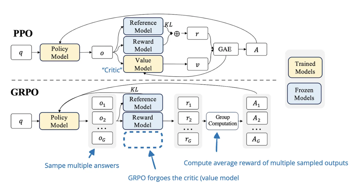
GRPO does this by simplifying value estimation: instead of a learned value function, it assigns the same baseline to every token in an episode, estimated via a Monte Carlo estimate over multiple completions ($a_{i,j}$) and their rewards ($r_{i,j}$), sampled from the same initial prompt/state ($s_i$).

A training step works on a batch of $N$ prompts $s_1, \ldots, s_N$. Note that the subscript has changed meaning: from here on it indexes a prompt in the batch, not a timestep, so $s_i$ is the $i$-th prompt (an initial state) rather than the state after $i$ tokens. For each prompt $s_i$, GRPO samples a group of $G$ completions $a_{i,1}, \ldots, a_{i,G}$ from the old policy $\pi_{\theta_{\text{old}}}$. $G$ is the group size, and three indices matter below: $i = 1, \ldots, N$ runs over prompts in the batch, $j = 1, \ldots, G$ runs over completions in that prompt’s group, and $t = 1, \ldots, T_{i,j}$ runs over the tokens inside completion $j$.

The split between the last two is the thing to hold onto, because the two halves of the objective live at different levels. The importance ratio is per token: writing $a_{i,j,t}$ for the $t$-th token of completion $j$ and $a_{i,j,<t}$ for the tokens before it,

so a completion of $T_{i,j}$ tokens contributes $T_{i,j}$ separate ratios.¹⁵ The reward and the advantage are per sequence: the reward is scored on the finished completion, so there is a single $A_{i,j}$¹⁶ for completion $j$ and every token in it is pushed by that same number.

Putting the levels together, and estimating the expectations by the batch itself, the objective (or loss) is:

Both averages are Monte Carlo estimates, which is why this is an $\approx$ and not an $=$. The objective is an expectation over two draws: which prompt comes out of the training set, and which group of $G$ completions the old policy happens to produce for it. The batch estimates the first with $\frac{1}{N}\sum_i$ and the second with $\frac{1}{G}\sum_j$. Everything from here to the end of the section happens inside one prompt’s group, with $i$ along only to say which prompt’s.

Concretely, if completion $j$ of prompt $s_i$ is “The answer is 12”, tokenized as $a_{i,j,1} = \text{The}$, $a_{i,j,2} = \text{ answer}$, $a_{i,j,3} = \text{ is}$, $a_{i,j,4} = \text{ 12}$, then $T_{i,j} = 4$ and that completion contributes four ratios $\rho_{i,j,1}, \ldots, \rho_{i,j,4}$, each multiplied by the same sequence-level advantage $A_{i,j}$.

To make an update meaningful, the advantage $A_{i,j}$ is computed by subtracting this baseline from the reward. A positive advantage means the response was better than expected, so its probability should increase; a negative advantage means it was worse than expected, so its probability should decrease.

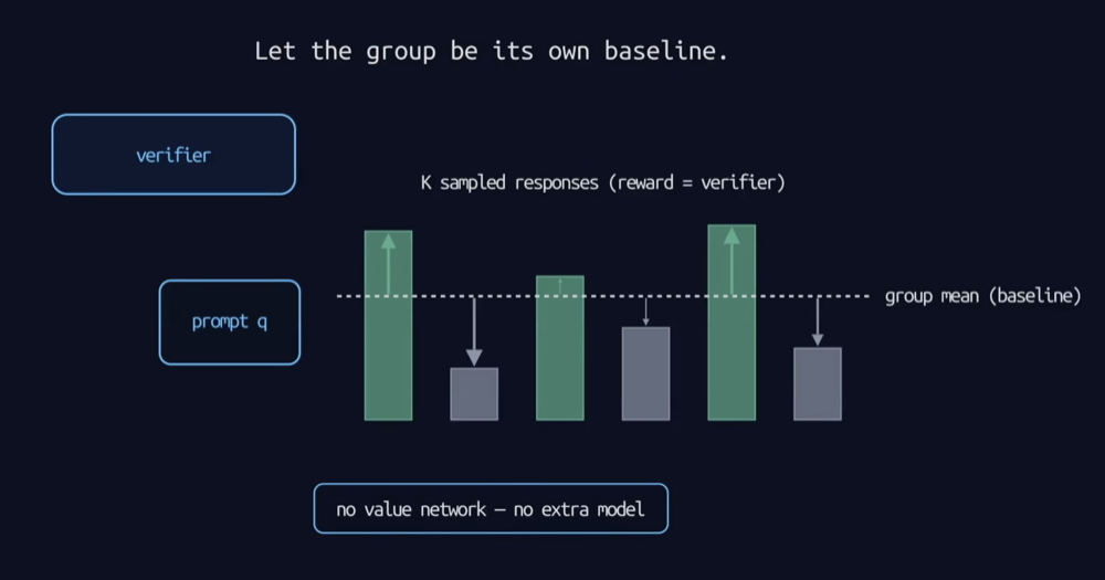
In PPO, the baseline comes from a learned value function. GRPO instead gets it from the group itself, using the rewards $r_{i,1}, \ldots, r_{i,G}$ of the completions sampled for prompt $s_i$:

Completions that score above the group average get a positive advantage and become more likely; completions that score below average get a negative advantage and become less likely. The model is always learning relative to itself, not some externally defined standard.

One thing the notation hides: $\pi_{\theta_{\text{old}}}$ is not the model as of the previous gradient step. It is frozen when the group is sampled and left alone while several gradient steps run against that group, so on the first of those steps $\rho_{i,j,t} = 1$ exactly, and it drifts away from 1 only as $\theta$ moves off the snapshot that produced the completions. $A_{i,j}$ is frozen the same way: the mean and standard deviation that define it were computed from the rewards of $\pi_{\theta_{\text{old}}}$‘s own samples, so every step taken on this group reuses the same $A_{i,j}$. Advantages are recomputed once per rollout group, not once per optimizer step. PPO’s inner loop works the same way, spelled out above.

Reinforcement Learning with Verifiable Rewards (RLVR)

The training method for these models, Reinforcement Learning with Verifiable Rewards (RLVR)¹⁷, proceeds very similarly to RLHF, but it makes the reward model optional in lieu of a scoring function that returns a positive reward when the answer is correct and 0 otherwise.

RLHF collects human preference data, trains a reward model on it, then optimizes the policy against that proxy. RLVR skips all of that when you have a ground truth to check against: the reward signal is the ground truth itself, not a learned approximation of it.

This can be seen as an RL feedback loop where, instead of a reward model, a verification function scores the agent’s completions.

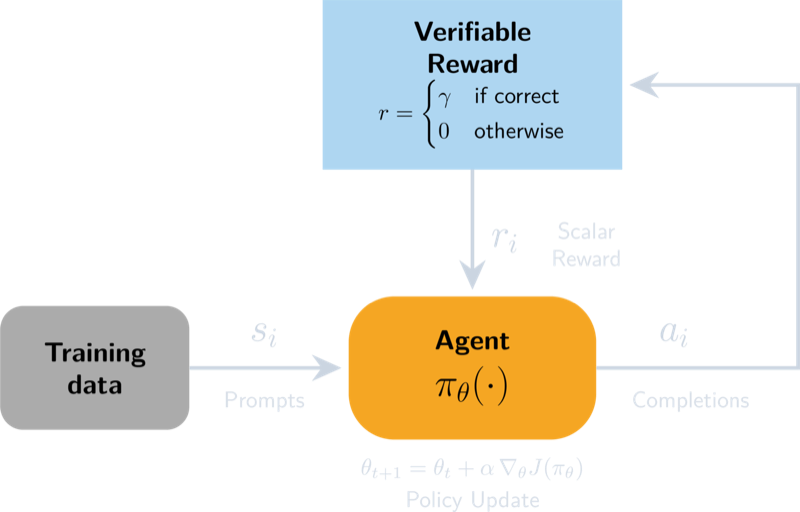
See below to see how different it is to score responses for RLHF versus RLVR. In RLHF, a reward model must evaluate subjective qualities. In contrast, RLVR uses verification functions that return definitive scores.

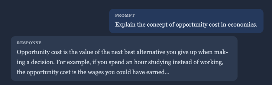
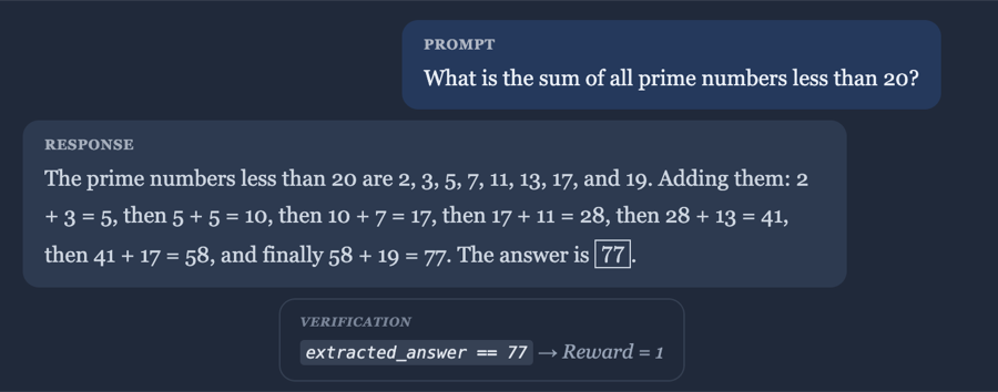
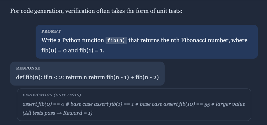
One motivation here is to avoid noisy or expensive human or learned rewards by using automatic correctness checks as the supervision signal during RL. The other is cost: by using “cheap” tools like calculators, we replace both the expensive reward model training and the reward model itself. Since the reward model is usually a whole pre-trained model with a regression head on top, dropping it makes RLVR much more efficient.

DeepSeek-R1 used RLVR with GRPO, which eliminates two expensive models from the training procedure, the reward model and the value model (critic), as illustrated in the figure below.

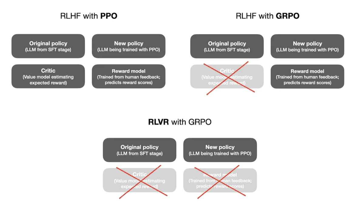
Unlike RLHF, there is no reward model to train, no reward model to overfit, and no proxy misalignment to worry about. But this only works when correctness is cleanly verifiable: for tasks where quality is subjective or multi-dimensional, you are back to needing a learned reward.

Large reasoning models

RLVR and GRPO can be used to improve the reasoning capabilities of LLMs on verifiable tasks, and research on this topic has led to the creation of large reasoning models (LRMs). The key distinction between an LRM and a standard LLM is the ability to dynamically “think” about a prompt prior to providing a final output. By increasing the length of the thinking process, these LRMs can use inference-time scaling, simply spending more compute on generating a completion, to improve their performance.

Architecturally, an LRM and a standard LLM are identical; the whole difference is in how they generate. Special tokens separate the thinking from the answer: the reasoning trajectory is generated first, wrapped between <think> tokens, and the model ends its reasoning process with a </think> token before proceeding to generate its final response.

LRMs also differ from standard LLMs in their training methodology. Both undergo similar pretraining and alignment phases, consisting of supervised finetuning (SFT) and RLHF. LRMs extend that standard process by performing large-scale RLVR on verifiable domains like math and code. Because verifiable reward signals are less prone to reward hacking, this RL training can be run at larger scale, meaning simply running it longer, with less risk of training collapse.

LRMs are not always the best tool to use, though. Because the training process for an LRM is focused on verifiable domains like math and code, its performance may be biased towards those domains, and away from non-verifiable ones like creative writing.

How DeepSeek-R1 Models Were Trained Using RL

The DeepSeek-R1 release was three kinds of model, differing in how much RL and SFT each one got:

1. DeepSeek-R1-Zero, trained with pure RL.
2. DeepSeek-R1, trained with instruction fine-tuning (SFT) and RL.
3. DeepSeek-R1-Distill variants, created via instruction fine-tuning (SFT) without RL.

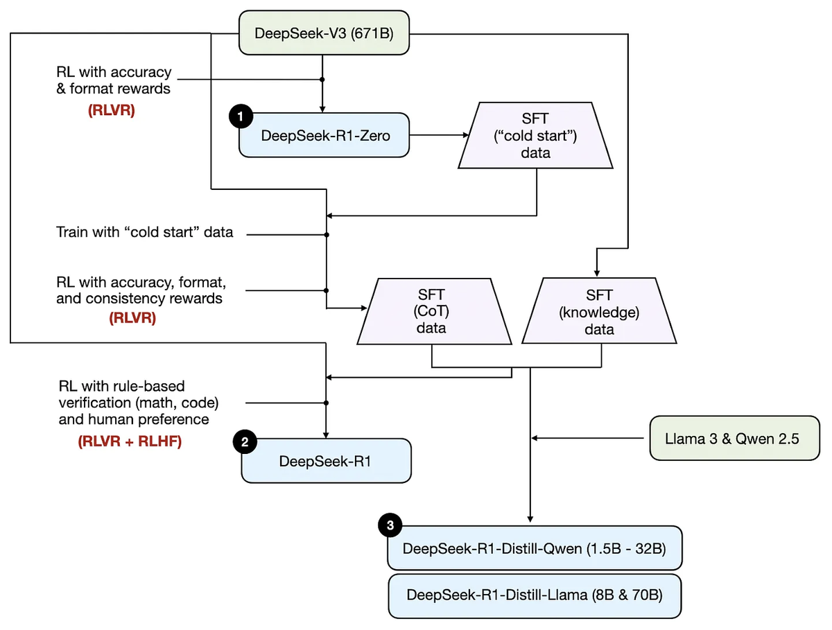
DeepSeek-R1-Zero was trained using verifiable rewards (RLVR) with GRPO, starting directly from the DeepSeek-V3 base model: no SFT stage and no human-preference reward model were used for it. That turned out to be sufficient for the model to exhibit reasoning abilities via intermediate-step generation, showing that it is possible to skip the SFT stage altogether. The model improves its reasoning abilities through exploration instead of learning from examples.

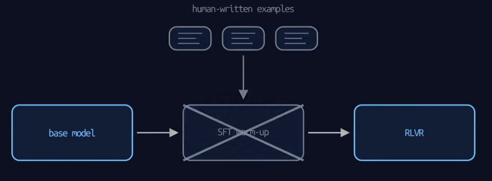
What it runs instead is a loop: sample completions from the current policy, check them with the verifier, update the policy on the result, and repeat.

Because there is no SFT stage, and training starts from the base pretrained model, the model has no idea what a good reasoning trace even looks like. Nobody ever showed it one. All it gets is the verifier’s verdict on the final answer.

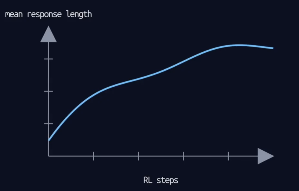
Nothing in the reward gives credit for length, yet the mean response length climbs on its own: longer reasoning chains help the model land on verifiable answers more often, and the verifier keeps rewarding that.

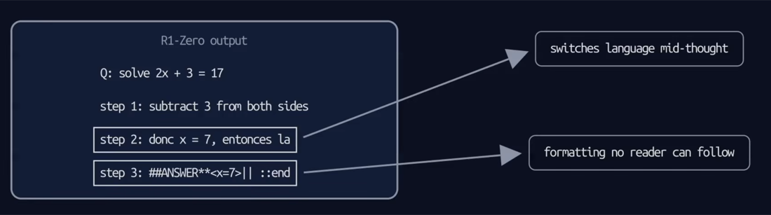
So R1-Zero proved reasoning could emerge from pure RL. The catch was that the output was hard to read. The model would slip between languages mid-thought, or produce formatting no human reader could follow. Nothing in the reward signal cared about readability, only correctness.

Emergent abilities from RL

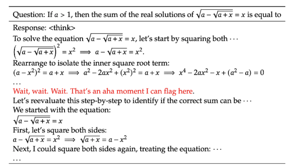
One of the most remarkable discoveries in R1-Zero’s training was the emergence of a phenomenon known as the “Aha Moment”, somewhat similar to how humans experience sudden realizations while problem-solving. It works like this:

1. The model makes an initial attempt at solving a problem.
2. It recognizes potential errors or inconsistencies.
3. It adjusts its approach based on that recognition.
4. It can explain why the new approach is better.

This ability emerged naturally from RL training, without being explicitly programmed, demonstrating learning rather than mere memorization of a process from the training data.

More detail on all of this is in the Hugging Face LLM course’s chapter on the breakthrough aha moment.

DeepSeek-R1 is the flagship model, the one with the best performance. The difference compared to DeepSeek-R1-Zero is that they alternated instruction fine-tuning, RLVR, and RLHF. The paper demonstrated clearly that supervised fine-tuning followed by reinforcement learning outperforms RL alone.

The fundamental claim behind DeepSeek-R1 and R1-Zero is that RLVR explicitly induces reasoning capabilities. However, recent findings suggest that reasoning behaviors, including the “Aha moment” described above, might already be present in base models because of pre-training on extensive chain-of-thought data. One critical study finds that DeepSeek-V3-Base already exhibits an “Aha moment” before any RL, and attributes the reasoning of some base models to pretraining biases.[1] A separate line of work plants deliberate errors in reasoning chains and measures whether the model catches them, finding that self-reflection and self-correction emerge progressively throughout pre-training, across various domains and model sizes.[2] Both further complicate attributing reasoning capabilities solely to RL.

A broader evaluation of RLVR reaches the same conclusion by looking beyond pass@1, comparing base and RLVR-trained models across model families, RL algorithms, and math, coding, and visual-reasoning benchmarks.[3] RLVR models usually do better on pass@1, meaning they are more likely to produce a correct solution on the first attempt. But pass@k counts a problem as solved if any of $k$ sampled answers is correct; at large values of $k$, commonly 128–1024, base models often solve more distinct problems than their RLVR counterparts. The authors argue that current RLVR therefore improves sampling efficiency by shifting probability toward rewarded reasoning paths that the base model could already produce, rather than teaching fundamentally new reasoning patterns. Off-policy distillation is different: supervised fine-tuning on trajectories from a stronger teacher can transfer patterns outside the student’s original reasoning distribution and expand what it can solve.

Zhou et al. (2023) call this broader view the Superficial Alignment Hypothesis in LIMA: Less Is More for Alignment.[4] The hypothesis says that knowledge and capabilities are learned primarily during pre-training, while alignment mostly teaches the model which behaviors and response formats to produce. LIMA fine-tunes a 65B LLaMA model on only 1,000 carefully curated examples, without reinforcement learning or human preference modeling, and finds that this small dataset is sufficient to teach strong instruction following and response formatting. From this perspective, RLVR’s pass@1 gain is an alignment effect: it makes an existing correct reasoning path more likely to appear.

Taken together, the evidence suggests a distinction between exposing capacity and expanding it. Current RLVR reliably turns latent reasoning into reliable behavior, but does not necessarily expand the model’s underlying reasoning boundary. In short, RL only shapes behavior; it does not teach new knowledge well. Distillation can expand that boundary by directly supplying new chain-of-thought patterns, and pre-training on data that contains such patterns may do the same before post-training begins.

Issues That Come Up for RL for LLMs

1. Policy entropy collapse

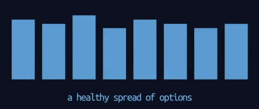
Reinforcement learning improves a policy by exploring alternatives, but every reward also concentrates probability on what already worked. If that concentration goes too far, exploration dies. That failure is policy entropy collapse.

Early in RL training the policy is still exploring: for a given prompt it can generate many different reasoning paths, spreading probability across a wide range of next tokens. As RL runs, that exploration can quietly die. Instead of a healthy spread of options, probability collapses onto a single repeated token.

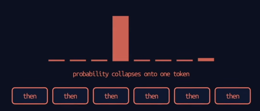
The policy has stopped exploring. It just repeats whatever already scores well, and once exploration is gone there is nothing left to discover.

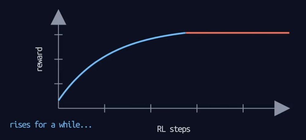
The reward curve rises for a while and then goes flat, not because the model solved the task but because it stopped trying anything new.

2. Objective bias from the normalization terms

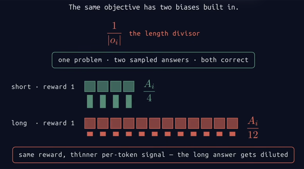
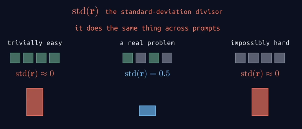
The bias here is not in the data, it is sitting inside the objective itself. The clean objective built above is not quite neutral. Look again at its two normalization terms, the $\frac{1}{T_{i,j}}$ that divides by response length and the $\text{std}(r_{i,1}, \ldots, r_{i,G})$ that divides the advantage by the group’s spread. Each one quietly bends the gradient in a direction that has nothing to do with whether the answer was right.

Length. Take two answers to the same problem, both correct, both earning a reward of 1, but one short and one long. Because the advantage is divided by the length of the response, the long answer’s signal gets diluted across more tokens. The optimizer reads that as “longer was better” and starts rewarding length for its own sake. That is not a signal about reasoning, it is an artifact of the math.

Spread. The standard deviation term does something similar across prompts. It overweights problems that are trivially easy or impossibly hard, where every sample in the group earns nearly the same reward, so $\text{std}(r)$ sits near zero and dividing by it inflates whatever tiny differences are left. The prompts that actually discriminate, where the group genuinely disagrees, get weighted down relative to those.

The fix from the Dr. GRPO[1] work is to recognize these as objective biases, properties of the loss itself rather than bugs in the data, and simply drop both normalization terms.

TODO: more issues to come.

GRPO vs GSPO

TODO: write this section, from “From GRPO to DAPO and GSPO: What, Why, and How”.

TODO

1. Refer to the Castform GRPO website.
2. RLHF Book: Reasoning
3. “The State of LLM Reasoning Model Training”, Sebastian Raschka
4. “Group Relative Policy Optimization (GRPO)”, Cameron R. Wolfe
5. “Direct Preference Optimization (DPO)”, Cameron R. Wolfe

Bibliography

- Zichen Liu et al., “Understanding R1-Zero-Like Training: A Critical Perspective,” arXiv preprint arXiv:2503.20783, 2025.
- Darsh J. Shah et al. (Essential AI), “Rethinking Reflection in Pre-Training,” arXiv preprint arXiv:2504.04022, 2025.
- Yang Yue et al., “Does Reinforcement Learning Really Incentivize Reasoning Capacity in LLMs Beyond the Base Model?” in Advances in Neural Information Processing Systems (NeurIPS), 2025.
- Chunting Zhou et al., “LIMA: Less Is More for Alignment,” in Advances in Neural Information Processing Systems (NeurIPS), 2023.