Actor-Critic Methods
July 14, 2026 · Updated September 12, 2026
Contents
Actor-critic methods build on policy gradients: alongside the policy (the “actor”), they learn a value function (the “critic”) to judge how good the actor’s actions are, giving a lower-variance learning signal than the raw Monte Carlo returns used in vanilla policy gradient.
In one line: policy gradients observe what was good or bad, then do more of the good stuff; actor-critic learns to estimate what’s good or bad, then does more of the good stuff. Same recipe, just swapping a noisy observation for a neural network’s own estimate of the value function.
Motivation: policy gradient makes inefficient use of data
Even with reward-to-go, which already stops an action from being blamed for rewards that came before it, policy gradient still only has one sampled rollout to learn from. Whatever happens after an action in that one particular trajectory still gets baked into its credit, whether or not it’s representative of what usually happens when the policy takes that action. Good and bad actions inside the same trajectory end up reinforced or punished together.1
This is sharpest under sparse rewards, where the only nonzero signal arrives once, at the very end of the episode. Two trajectories that make very different amounts of real progress toward the goal, but happen to land on the same final reward, get treated as equally good, or equally useless. The algorithm has no way to see the difference.2
All policy gradient ever knows is that a trajectory succeeded or failed as a whole; it has no notion of how good any specific state or action was on its own. That is exactly the gap a learned critic is built to fill: an estimate of a state’s or action’s expected future reward, averaged over the policy’s actual behavior, rather than one noisy, one-off realization of it.
Preliminaries
- value function : the future expected reward starting at state and following policy from there
- Q-function : the future expected reward starting at state , taking action , then following policy from there
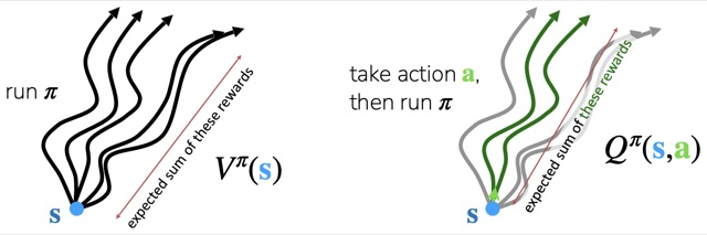
and are related: since is the expected future reward under ‘s own behavior at , it must equal averaged over the actions would actually choose at ,
answers “how good is action ,” while answers “how good is state , on average, under ‘s own choices.” Averaging the first over ‘s action distribution gives the second back.
This gives a natural way to measure how good a specific action is relative to the policy’s own average behavior: the advantage function,
how much better (or worse) it is to take action than to follow ‘s own behavior at state .
From reward-to-go to Q: a lower-variance estimator
Recall the reward-to-go estimator,
This update increases the probability of actions that led to large future rewards. But is only ever computed from one sampled rollout: it’s an estimate of the future reward, not the future reward itself. The same first action can lead to wildly different futures.
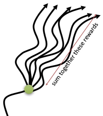
This is exactly the high variance from the motivation above, made concrete: swings with whichever future happened to get sampled, even though the action itself, taking at , is the same every time.3
A better estimate averages over every possible future after taking in , instead of relying on the one future that happened to get sampled:
This is exactly the -function defined above: the expected future reward from taking at and then following . Substituting for the sampled reward-to-go gives a new, lower-variance estimator:
Instead of saying “this one rollout earned reward 8,” this says “this action is generally worth about 8”: the update is now driven by an averaged, expected value, rather than one noisy, one-off realization of it.
What the Q-function learns
Instead of trusting a single rollout, the critic accumulates experience across many episodes: every time the policy takes action at state , it records the return that followed, and averages over all of them.4 This average is exactly the Monte Carlo estimate of defined above, just computed from many rollouts instead of one.
Suppose that after enough episodes, this average settles at . The policy update no longer uses the reward of that one sampled rollout happened to return; it uses , the critic’s running average over everything it has seen.
Q still depends on the state, not just the action
Even has a subtle flaw: it mixes together how good the state already is with how good the specific action is. In a position that’s already winning, every legal move can look great under , not because any one move is exceptional, but because the state itself already guarantees a good outcome.5
The fix is to stop asking “is this action good?” in absolute terms, and instead ask “is this action better than what I usually do from this state?” That’s exactly what the advantage function measures: subtracting off the state’s own average value, , removes whatever part of was just “the state is good,” leaving only the part attributable to the action itself.6
Plugging into the gradient in place of gives the actor-critic estimator:
Better estimates of lead to less noisy gradients. The actor no longer chases large absolute rewards caused by simply being in a good state; it updates based on whether an action was better or worse than expected from that specific state, a more stable and efficient learning signal.
The actor-critic loop
Fitting , , or turns actor-critic into a small extension of the online RL loop: collect a batch of data with the current policy, fit a model to estimate the expected return, then use that fitted estimate to improve the policy.
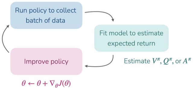
You estimate value metrics like the State-Value , Action-Value , or the Advantage (which is seen in the top equation). This gives you the ground truth weight needed for your gradient update.
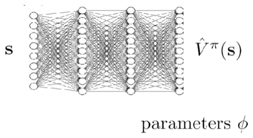
In practice, this fitted model is a neural network: it takes a state as input and outputs an estimate , with its own parameters , separate from the policy’s parameters .
Training the value network
Fitting turns into an ordinary supervised learning problem: for every state visited in a batch, use the observed return , the actual reward-to-go collected from that state onward, as the regression label.
- input: the state
- target: the observed return
The loss is standard mean squared error between the network’s prediction and this target,
training by gradient descent on , exactly like any other regression problem.7
Every episode that passes through a given state contributes another noisy sample of the return from there. Training on many of these samples pushes the network’s prediction toward their average, which is exactly : the expected return under , not any single episode’s realization of it.8
Bootstrapping: expressing Q with just V
Fitting a network for alone, without a separate -network, is enough. Start from written as a sum of expected future rewards, and pull out the very first one, the reward that arrives immediately after taking :
Everything after the first reward is, by definition, exactly : the expected future reward from following starting at the next state. There’s an expectation, , because after your action, many next states are possible. But in reinforcement learning we only ever experience one next state per rollout: current state, action, observed next state, no branching. So the last line approximates that expectation with the one sampled next state: it plugs in evaluated at the that was actually observed, instead of averaging over all of them.
This is called bootstrapping: using the current value estimate itself to stand in for future rewards, instead of needing a whole separate rollout (or a model of the environment’s dynamics) to know what happens next.
Substituting this into the advantage function, :
No -network required: the advantage, which needed a moment ago, can now be computed from alone, plus the one reward that was actually observed.
Temporal difference learning: bootstrapped targets
The Monte Carlo target used above, , has a practical problem: you can’t compute it until the episode is over. If an episode runs for steps, the network can’t take a single gradient step until step .
The fix is the same bootstrapped estimate derived above, now used as the training target itself, instead of just for the advantage:
Instead of waiting for the rest of the episode, the label is available immediately: one observed reward, plus the network’s own current guess at everything after it.9
At first, that guess can be quite wrong. But every gradient step improves a little, which means every subsequent target gets a little more accurate too: the network is teaching itself, bootstrapping better and better labels out of its own improving predictions.
The loss function doesn’t change at all, only the target does:
Learning is now much faster, since it no longer waits for an episode to end.
This is called temporal difference (TD) learning because of what’s being compared: the current prediction , against a target built from the next time step, . Their difference is the TD error,
If , the state turned out better than expected, so should increase. If , it turned out worse than expected, so should decrease.
Bias vs. variance: Monte Carlo vs. TD
The Monte Carlo target from training the value network and the bootstrapped TD target above sit on opposite ends of a classic tradeoff.
The Monte Carlo target, , uses the actual future return realized in that one sampled episode. It’s unbiased: averaged over enough episodes, it converges to the true . But it’s noisy, since a single episode can be lucky or unlucky, so the label attached to any one state can swing widely from episode to episode.
The TD target, , uses the current, imperfect estimate in place of the true value of the next state. Since can be wrong, especially early in training, this introduces bias: the target itself may be systematically off. But it only depends on one sampled reward, not an entire trajectory’s worth of randomness, so it has much lower variance.
- Monte Carlo: unbiased, high variance
- TD: some bias, lower variance
Monte Carlo trusts the data completely and pays for it in noise; TD trades some of that noise away by trusting its own, imperfect predictions instead.10
N-step returns: a middle ground
Monte Carlo and 1-step TD are two ends of a spectrum: sum every real reward all the way to , or bootstrap after just one. Nothing forces that choice to be so extreme.
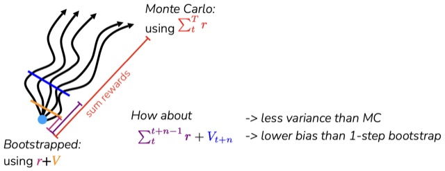
An n-step return sums the actual, observed rewards for the first steps, then bootstraps off for everything after that:
recovers the 1-step TD target from above; recovers the Monte Carlo target, with no bootstrapping at all.
In practice, some strictly in between, , often works best: using real rewards before bootstrapping means less of the estimate leans on being correct, so it has less variance than Monte Carlo; but it also depends on fewer of the single sampled trajectory’s rewards than the full return does, so it has lower bias than the 1-step bootstrap.
A full algorithm walkthrough
Putting every piece together needs one last bit of notation: the discount factor , which weights rewards further in the future slightly less than immediate ones (everywhere above has implicitly used ). With it, the actor-critic algorithm is:
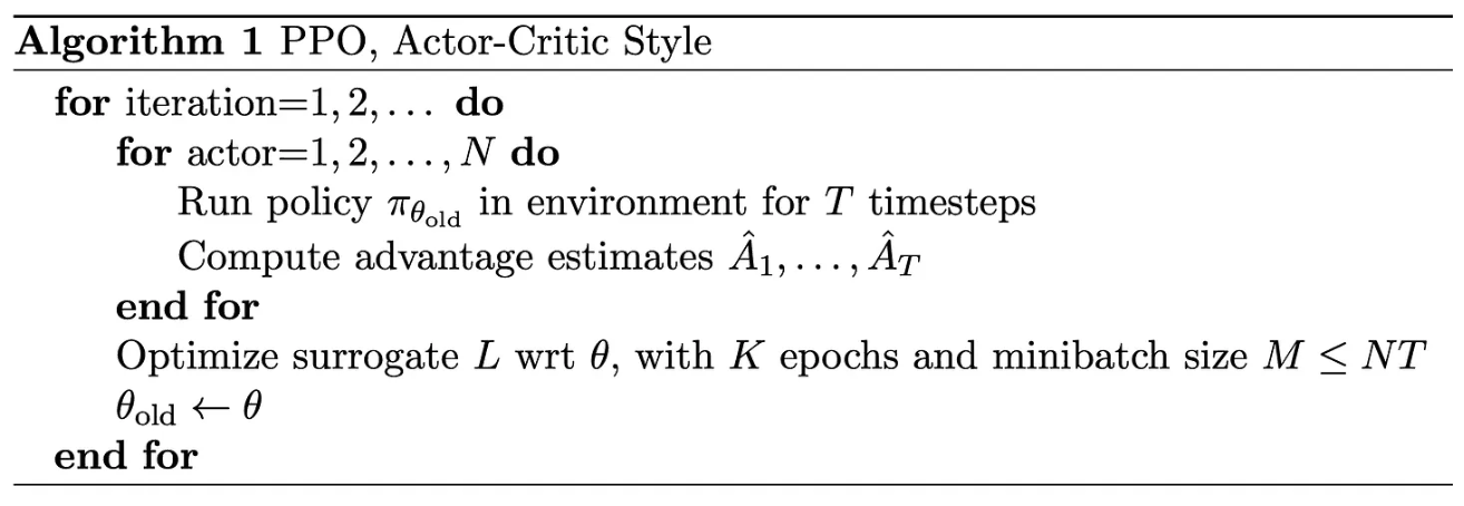
- Sample a batch of trajectories by running the current policy .
- Fit to the summed rewards in the batch.
- Evaluate the advantage at every timestep,
- Evaluate the policy gradient,
- Update the policy, .
Then repeat from step 1 with the newly updated policy.
Step 2’s target and loss are exactly the n-step return from above, now with discounting folded in:
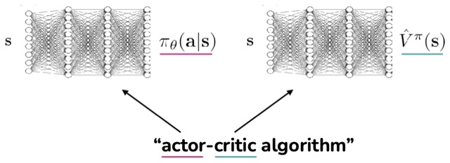
Steps 1 and 4 are the actor: the policy network , updated by the policy gradient. Steps 2 and 3 are the critic: the value network , whose bootstrapped estimate turns raw rewards into the advantage the actor learns from. Two separate networks, trained together, each taking the same state as input, giving the method its name.
Off-policy actor-critic
The algorithm above is on-policy: every gradient step needs a fresh batch of trajectories collected under the current policy , including the batch the critic is trained on. Turning this into an off-policy method means reusing data collected under an older policy for more than one gradient step, instead of collecting a batch, taking one gradient step, and throwing it away.11 Each transition gets reused many times instead of once, which is far more sample-efficient. Importance sampling is what makes that reuse valid, at the cost of a slightly stale advantage estimate.
Version 1: Multiple Gradient Steps
- Sample a batch of trajectories by running the current policy .
- Fit to the summed rewards in the batch.
- Evaluate the advantage at every timestep,
- Evaluate the importance-weighted policy gradient,
- Update , then repeat from step 4 for another gradient step on the same batch.
This is what gives the version its name: instead of one gradient step per batch, steps 4 and 5 loop several times on before the outer loop ever touches step 1 again. But the advantage being reused in every one of those inner steps is still exactly what step 3 computed, from the old policy ; it never gets recomputed as moves. The more inner steps you take, the more outdated that advantage becomes, and the less it reflects what would actually experience now. can’t wander too far from before this stops being reliable: once the two policies disagree enough, the importance weights also blow up, exactly the failure mode trust regions exist to prevent. In practice, “multiple” here means a handful of steps, not many.
After a handful of these inner steps, set and repeat from step 1 with a freshly collected batch.
Version 2: Replay Buffers
[Update this]
Proximal Policy Optimization
Recall the surrogate objective trick from policy gradients: instead of writing out a full gradient by hand, define a scalar objective whose gradient recovers it, so a single backward() call does the work. Applying that here, to the importance-weighted update from off-policy actor-critic, gives the surrogate objective
Differentiating with respect to , treating as a constant, gives back exactly that importance-weighted policy gradient. As always, climbing increases the probability of high-advantage actions and decreases the probability of low-advantage ones.
has two pieces. The importance ratio,
compares the new policy to the old one. Unpacking each symbol:
- is the current state. For an LLM, that’s the prompt plus the tokens generated so far.
- is the action. For an LLM, usually the next token, or sometimes the entire generated sequence.
- is the old policy: the model as it was before the update.
- is the new policy, the one being trained.
- is the probability the policy assigns to taking action in state .
So means behaves exactly like ; means is more likely to take this action than was; means less likely.12 The advantage, , was computed once from the old policy’s data: positive means the action was good, negative means it was bad. Multiplying them together says: increase the probability of good actions, decrease the probability of bad ones.
Why multiple gradient steps can go wrong
Version 1 already flagged the risk of repeating steps 4 and 5 too many times: nothing in itself penalizes for drifting far from , so an optimizer that’s free to keep climbing will happily push far past , long after the advantage estimate it’s multiplying has stopped being trustworthy.13
TRPO fixes this by directly constraining how far is allowed to move, measured by KL divergence: . It works well, but solving a constrained optimization problem at every gradient step is mathematically involved.
PPO takes a simpler route: instead of constraining the policy directly, just stop the importance ratio itself from getting too large.
Clipping the importance ratio
Pick a small (commonly ), and clip to the interval before it’s allowed to multiply the advantage: anything outside that interval gets pulled back to the nearest edge.14
Clipping matters because, left alone, grows without bound: for a fixed positive advantage, a bigger ratio always means a bigger objective, so the optimizer is rewarded for pushing arbitrarily far from . Once the clipped ratio hits its boundary, it stops growing, so there’s no more reward for pushing it any further.15
The PPO objective
Taking the smaller of the clipped and unclipped versions, then summing back over the sampled timesteps the way did, gives the full PPO objective:
where is the importance ratio at a single sampled state-action pair. The and the clip both apply per sample, inside the sum: every term is capped on its own before anything is added up. The PPO paper writes this same objective as , with an expectation over samples in place of the sum.
Why take the minimum, instead of just always optimizing on its own? Because clipping alone can accidentally reward exactly the policy changes it’s supposed to discourage: whenever has moved outside the trust region in a bad direction, the clipped term can score better than the true, unclipped one. Taking the minimum always keeps whichever number is worse, so a bad update can never be made to look better than it actually is.16
Either way, the policy can’t change too much in a single update while still improving the objective. This clipping mechanism, simple to implement and no constrained optimization required, is the core idea that makes PPO both stable and simple compared with earlier trust-region methods like TRPO.
For what this algorithm looks like once the environment is an LLM emitting tokens, a single token’s update worked end to end, the KL penalty against a reference model, and what “the old policy” means in practice, see PPO for LLMs.
The count behind , , and is easiest to see in a concrete example.17
TODO: add Generalized Advantage Estimation (GAE).
Footnotes
-
Consider a robot walking, where a good start is undone by one bad step:
Step Action Outcome 1 forward ✓ 2 forward ✓ 3 backward ✗, robot falls The trajectory’s total reward is bad, because of the fall. Vanilla policy gradient only sees that one bad number for the whole trajectory, so it decreases the probability of every action in it, forward included: it pushes down the likelihood of stepping forward. But the first two forward steps were good; only the backward step at step 3 caused the fall. Policy gradient can’t tell the two apart, because both actions get scored by the same trajectory-wide outcome. ↩
-
Consider three attempts by a robot to fold a jacket, with reward given only at the very end of the episode:
Trajectory Outcome Reward Folds only the sleeves Flattens the jacket but doesn’t fold it Folds it completely Policy gradient only sees the reward column: gets reinforced, while and are both treated as equally useless failures. But and each made real progress toward the goal; the algorithm has no way to see that, because the only feedback it ever gets is the final number. ↩
-
Suppose taking action at state could lead to four possible future paths:
Path Reward A B C D Vanilla policy gradient only ever samples one of these paths per rollout. If it happens to observe path B, it sees a reward of and credits accordingly. But that doesn’t mean is only worth . ↩
-
Suppose the critic has recorded the return that followed taking action at state , across several episodes:
Episode Return 1 2 3 4 5 6 7 Averaging over all of these episodes,
a single noisy sample (episode 1’s return of ) is far from this average; the critic’s job is to converge toward , not toward whatever any one episode happened to return. ↩
-
Suppose you’re playing chess in an already-winning position, with three legal moves, every one of which still leads to a win:
Move -value Queen Bishop Pawn All three numbers are large mostly because the state is already fantastic, close to a guaranteed win, not because any individual move is exceptional. Using directly would credit all three moves with a huge update, even though none of them is meaningfully better than the others. ↩
-
Continuing the chess example above, the state’s value is the average -value over the three moves, . Subtracting it out gives each move’s advantage:
Move -value Queen Bishop Pawn Instead of three huge, nearly identical rewards, the advantage shows Queen is mildly better than average, Bishop is exactly average, and Pawn is mildly worse, a much more informative signal than , , and . ↩
-
Suppose the network currently predicts for some state, but the observed return from that state was . The loss is . After enough gradient steps on examples like this one, the prediction gradually climbs toward the target:
↩Step Prediction Before training After some training After more training Eventually -
Suppose state shows up across five different episodes, with observed returns , , , , and . The network sees the training pairs , , , , , one per episode. Minimizing squared error across all of them pulls the prediction toward their average, , so the network learns , close to the state’s true expected return. ↩
-
Suppose the immediate reward is , and the network’s current prediction for the next state is . The bootstrapped target is , available right away, without waiting to see how the rest of the episode plays out. ↩
-
Consider two episodes running through the same two states, Pink and Blue, before reaching a terminal:
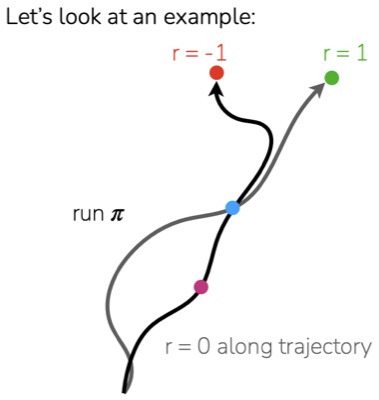
Source: Stanford CS224R. - Episode 1: Blue Green ()
- Episode 2: Pink Blue Red ()
Estimate Value Why Blue was visited twice, with returns and . Average . Pink was visited only once, and that episode ended at the red terminal. Return . Blue is followed by a different state in each episode, Green in episode 1, Red in episode 2, and both are terminal, so . Its TD target in episode 1 is ; in episode 2 it’s . Blue sees both targets over training, and gradient descent on the two squared errors pulls its estimate toward their average, . The TD target for Pink is , since Blue has already learned a value of after the two episodes. The key difference: Monte Carlo uses the actual return from the episode, while TD uses the immediate reward plus the estimated value of the next state. That’s why : it saw the whole bad outcome. But : it only looks one step ahead to Blue, whose estimated value is already . ↩
-
Without off-policy learning: collect data, take one gradient step, discard all the data, collect again. Every transition is used exactly once, no matter how expensive it was to collect. With off-policy learning: collect data once, then take a gradient step, another, another, another, and only then collect more. Each transition gets reused across every one of those steps instead of being thrown away after a single update. ↩
-
Suppose the state is the prompt “The capital of France is”, the action taken during rollout was the token
Paris, and the old policy assigned it :Next token Old policy ParisLondonRomeAfter a training step, the new policy predicts:
Next token New policy ParisLondonRomeThe ratio for the action actually taken is : the new policy makes
Paris25% more likely than before. Suppose instead the new policy had predictedParis,London,Rome. Then , and the chosen action is only half as likely as it was under the old policy.Which direction is desirable depends on the sign of the advantage. With , a larger ratio increases the objective, so the optimizer is encouraged to raise this action’s probability. With , raising the probability hurts the objective, and the optimizer pushes the ratio below instead. ↩
-
Suppose the old policy is Left , Right , and the advantage says . The optimizer keeps increasing the probability of Left. After several gradient steps: Left , Right . The importance ratio for Left is now . Left unchecked, further optimization pushes to , , , , and beyond: becomes very different from the that generated the advantage estimate, so the optimizer ends up trusting information that’s no longer accurate. ↩
-
With , the clipping interval is :
Raw ratio Clipped Anything outside gets pulled back to the nearest edge; anything already inside passes through unchanged. ↩
-
Suppose the advantage is . Without clipping, the objective grows without bound as the ratio grows:
Ratio Objective With clipping applied first:
Ratio Clipped Objective Once the ratio passes , the clipped objective stops growing: there’s no more reward for increasing the probability any further. ↩
-
Compare against always optimizing just on its own, with (clip interval ):
- Good action, ratio too high: , . Unclipped ; clipped . , exactly what clipping alone would give. Here the changes nothing.
- Bad action, ratio too high: , (a bad action made much more likely). Unclipped ; clipped . Since , always using the clipped objective would score this update , better than it deserves, effectively rewarding the bad update for landing outside the clip region. PPO’s refuses that, keeping the worse, true score.
- Good action, ratio too low: , (a good action made much less likely). Unclipped ; clipped . Always using the clipped objective would score this , again better than it deserves. PPO’s keeps the worse score instead.
- Bad action, ratio correctly reduced: , (a bad action correctly made much less likely). Unclipped ; clipped . : PPO still applies the more conservative, clipped score here, even though this particular change was in the right direction. Once moves outside the trust region, the objective saturates, whether or not that move happened to be beneficial.
In every case, the either matches the clipped objective, when clipping alone already handles the update correctly, or falls back to the true, unclipped score, when clipping alone would have flattered a bad update. That’s what stops the clipped objective from ever making an undesirable policy change look better than it is. ↩
-
Suppose actors each contribute one rollout, and the implementation groups 10 whole rollouts into each minibatch. One optimizer step processes 10 rollouts, so one epoch contains optimizer steps and processes all 100 rollouts once. With , optimization takes steps and accounts for rollout-usages. These are not 400 unique rollouts: the same 100 are reused once in each of the four epochs. Only after all four epochs does PPO discard that batch, refresh the old policy, and collect new rollouts. ↩