Policy Gradients
July 12, 2026 · Updated August 30, 2026
Contents
Policy gradient methods are a class of reinforcement learning algorithms and a sub-class of policy optimization methods. Unlike value-based methods, which learn a value function to derive a policy, policy optimization methods directly learn a policy function that selects actions without consulting a value function. For policy gradient to apply, the policy function is parameterized by a differentiable parameter .1
Preliminaries: RL and MDPs
Reinforcement learning is about an agent interacting with an environment: at each time step the agent observes the state of the world, takes an action, and the environment responds with a reward and the next state.
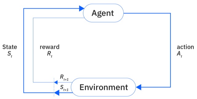
The formalism behind this loop is the Markov decision process (MDP): a mathematical model for sequential decision making when outcomes are uncertain. It can be formulated as
a state space , an action space , transition probabilities , and a reward function . The basic objects:
- state : the state of the “world” at time
- action : the decision taken at time
- trajectory : sequence of states/observations and actions
- reward function : how good is ?
- policy (or from observations): the behavior, usually what we are trying to learn
For a trajectory , the return is the sum of rewards collected along it:
We want policies that generate high-return trajectories.
RL methods split by where their training data comes from:
- offline: using only an existing dataset, no new data from the learned policy
- online: using new data from the learned policy
This note only covers the online case.
Online RL
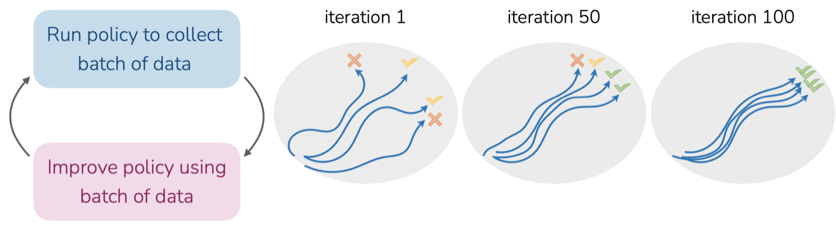
Online RL is a loop: run the current policy to collect a batch of data, improve the policy using that batch, and repeat. Over iterations, the policy’s trajectories concentrate on the behaviors that earn reward.
Policy Gradient objective
Goal: learn a policy that maximizes the expected sum of rewards over all possible episodes that this policy could produce:
where the trajectory distribution factorizes as
This factorization is the Markov property: the next state depends only on the current state and action, not on the rest of the history.
The expectation inside the objective is usually named , the objective function:
tells us how good the policy is: a higher means a better policy, and .
Computing exactly isn’t possible, since there are millions (or infinitely many) possible trajectories due to randomness in the environment’s transitions and the policy’s action choices. (We’ll see how to get around this with Monte Carlo approximation further below.)
Using the return defined above, this is just . Writing out the expectation over the trajectory distribution gives an equivalent, integral form of the objective:
To improve the policy using the batch of data we collect with it, we want the gradient , because gradient ascent will update
Taking the gradient:
Move the gradient inside the integral:
But is difficult to work with. We don’t know how to directly estimate gradients of trajectory probabilities.2
The log-derivative trick rewrites this into something we can estimate. Since
multiplying both sides by gives
Substituting this into the gradient, we replace with :
This now looks like an expectation, since . Therefore
Intuitively, this term reweights the policy update by how good the trajectory turned out to be.3
This can be estimated using Monte Carlo approximation. A fundamental fact from probability: if , then
for samples drawn from . After collecting trajectories by running the policy,
is an unbiased estimate of .
Going back to the original gradient integral, : why couldn’t we have estimated that one directly with Monte Carlo, instead of going through the log-derivative trick?4
We don’t need the environment dynamics
can be expanded further. Using the trajectory factorization,
and differentiating with respect to :
since the initial state distribution and the environment dynamics don’t depend on , only the policy does, so their gradients vanish. This is a huge simplification: computing no longer requires knowing the environment’s transition probabilities at all, only the policy’s own log-probabilities, which we have direct, analytical access to. The gradient and its Monte Carlo estimate become
Full algorithm
Putting it all together, this is the online RL loop from earlier, made concrete. This is the “REINFORCE algorithm,” the vanilla policy gradient:
Then repeat from step 1 with the updated policy.
This algorithm works, but it is noisy and has very high variance. A single lucky episode with a huge reward can dominate the gradient estimate.7
Reward-to-go: fixing credit assignment
One natural question comes up: why should an action at time get credit (or blame) for rewards that happened before it? Policy behavior at time can’t affect rewards at ; future actions cannot change the past.8
Causality says we should only weight by the rewards that came after it, not the whole trajectory’s return. So we replace
with the reward-to-go,
giving a new estimator:
Before, every action in a trajectory was weighted by the same total return. Now, each action is weighted only by the rewards that came after it, the only ones it could have influenced. Removing this irrelevant past-reward noise decreases variance, while the expected gradient stays correct.9
Baselines: centering the reward
Even with reward-to-go, there’s still a problem.10 If every trajectory in a batch gets a similar, uniformly positive reward, REINFORCE increases the probability of all of them, even the relatively worst one, since it only looks at each trajectory’s raw reward, not how it compares to the rest of the batch.
To fix this, we introduce a baseline and subtract it from the reward:
A natural choice is the batch’s average reward,
so instead of weighting by , we weight by how much better or worse than average each trajectory did.11 This also reduces variance: rewards that used to be large, similar numbers become small numbers centered at zero, so the gradient magnitude no longer swings wildly from batch to batch.12
Subtracting a constant baseline doesn’t bias the gradient. In expectation,
so the estimator stays unbiased. (The full proof isn’t given here; see Stanford CS224R’s policy gradient slides.) The average reward is a pretty good baseline: unbiased, and lower variance.
Limits of baselines: sparse rewards
Even with a baseline, policy gradient still struggles when the reward is sparse, given only once at the very end of a trajectory. The baseline centers a trajectory’s total return around the batch average, but it can’t see inside the trajectory: two trajectories that happen to end with the same final reward get exactly the same weight, even if one made real progress along the way and the other made none at all.13
Because the reward is sparse, the gradient doesn’t know which specific action along the timeline was good or bad; it just scales the entire sequence of actions by the same final number. Policy gradient is still noisy and high-variance in this regime: even with a baseline, it struggles to tell “close failures” from “total failures” apart. Fixing this needs either dense rewards (small intermediate rewards for sub-steps toward the goal) or large batches, so the noise averages out over enough samples.
Implementing this efficiently: the surrogate objective
Putting reward-to-go and the baseline together, the full estimator is
Computing this naively means calling backward() once per state-action pair: differentiate , multiply by its own , and sum. That’s a lot of individual backward passes.14
Deep learning frameworks are built around a single scalar loss and one backward() call, not thousands of gradients accumulated by hand. So instead we construct a scalar surrogate objective : not the true objective , but a quantity whose gradient happens to equal the policy gradient we actually want:
comes from the environment and the batch of collected data, not from the network, so autograd treats it as a constant with no dependence on . Differentiating therefore only differentiates , carrying straight through:
which is exactly the policy gradient term above. A single backward() call on therefore gives the same gradient as summing every individual term by hand.15
is also exactly the term that shows up in maximum likelihood training: for classification, cross-entropy loss is . The policy gradient loss, , is the same thing weighted by , a weighted maximum likelihood that pushes up the log-probability of actions in proportion to how much better than the baseline they did.
In PyTorch, this is:
log_probs = policy.log_prob(actions)
loss = -(log_probs * advantages).mean()

optimizer.zero_grad()
loss.backward()
optimizer.step()
where advantages holds per timestep, and the sign is flipped since optimizers minimize by convention.
On-policy vs. off-policy
Every variant of the estimator covered so far, from vanilla REINFORCE through reward-to-go, the baseline, and the surrogate objective, shares one property: the expectation is over trajectories sampled from the current policy . But step 3 of the full algorithm changes . Once that happens, the trajectories used to compute that gradient no longer come from the policy we’re now trying to improve, so we have to go back to step 1 and collect a fresh batch under the new before taking another gradient step.
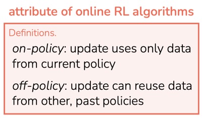
Every estimator above is on-policy: each gradient step needs its own brand-new batch of trajectories, and none of the old data can be reused once changes. That makes them sample-inefficient.
Importance sampling: reusing old trajectories
Being on-policy means all the old data is, technically, invalid the moment the policy changes: we need fresh rollouts under the new at every single gradient step, which is expensive. Importance sampling gives a way to reuse trajectories collected under an older policy instead.
The general trick: suppose we want an expectation under a distribution ,
but only have samples from a different distribution . Multiplying the integrand by ,
so an expectation under can be estimated from samples drawn from instead, as long as each sample is reweighted by the importance weight .
Applying this to the policy gradient objective: we want , the expectation under the current policy , but only have trajectories collected under an older policy . Importance sampling rewrites the objective as
so the old trajectories can be reused, each one reweighted by the correction factor : how much more (or less) likely that trajectory would be under the new policy than under the old one.
To compute this correction factor, recall the trajectory factorization , and likewise for the old policy, . Both trajectories were generated in the same environment, so the initial state distribution and the dynamics are identical top and bottom, and cancel out of the ratio:16
leaving only a ratio of policy probabilities. We never need to know the environment dynamics, only the old and new policies’ probabilities of the actions actually taken.17
Off-policy policy gradient
Combining reward-to-go, the baseline, and importance sampling gives a full off-policy policy gradient: update the latest policy using trajectories sampled from an old policy , instead of itself.
Start from the on-policy reward-to-go-with-baseline estimator, written as an exact expectation:
The problem: this expectation is over trajectories , sampled from the very policy we’re trying to update, exactly the data we don’t have.
Using importance sampling, rewrite the expectation over the old policy’s trajectory distribution instead, correcting each sample with the importance weight :
and substituting in the per-timestep form of that ratio,
This is now genuinely off-policy: it can be computed entirely from trajectories collected under the old policy , with no fresh rollouts under required.
But the product term, , is the catch: it multiplies per-timestep ratios together, and for longer horizons this product can become vanishingly small or explosively large, since even a small, consistent per-step difference between the two policies compounds multiplicatively over many timesteps.18
Reducing variance: per-timestep importance sampling
Because of this high-variance trajectory-level product, it helps to stop thinking about importance-sampling an entire trajectory at once, and instead importance-sample one timestep, one state-action pair, at a time.19 Instead of
consider
Write each timestep’s importance ratio as , and its gradient contribution as . The old, trajectory-level estimator, for a single trajectory, was
one giant product of ratios, multiplied by one giant sum of gradient contributions: every in the sum gets scaled by the same trajectory-wide weight. The new, per-timestep estimator is instead
Now every timestep carries its own weight. Instead of
we have
- step 1 → its own weight
- step 2 → its own weight
- step 3 → its own weight
- …
Each is scaled only by its own timestep’s ratio, not by a product of every ratio in the trajectory. This is exactly why per-timestep importance sampling reduces variance so dramatically.
But there’s a new problem: a policy doesn’t output directly, only . Expanding with the chain rule of probability, , splits into two factors:
The first factor, the ratio of action probabilities, is easy: both policies hand it to us directly. The second factor, the ratio of state marginals, is not. isn’t something either policy outputs: it’s the probability that the agent reaches state at all, which depends on the policy, every action taken before , and the environment’s transition dynamics, none of which we have direct access to.
In practice, this state-marginal ratio is just approximated as . If is only a small update away from , the two policies tend to visit nearly the same states, so and
This approximation only holds when the two policies are close together.
Substituting it back in gives a fully practical estimator:
The huge trajectory-length product is gone. What’s left is a single probability ratio per timestep, far more stable than multiplying together of them.
When does our off-policy approximation stop working?
The per-timestep estimator above leans on approximating , which quietly assumes hasn’t drifted far from .20 Once the new policy diverges enough, this breaks: the two policies start visiting different states, so the trajectories collected under no longer describe what would actually encounter.21
To keep the approximation valid, we can constrain how far a single update is allowed to move the policy: require the new policy to stay close to the old one, measured by KL divergence,
KL divergence measures how different two probability distributions are. If stays within of at every state, the old data stays relevant, the state-marginal approximation stays reasonable, and the resulting gradient estimate stays trustworthy.
This constraint shouldn’t be checked at a single state; it should hold on average, over the states the old policy actually visited:
Pick a small threshold , and reject (or shrink) any update that would push the policy further than that. This constrained-optimization idea, keeping every update inside a “trust region” around the old policy, is exactly what TRPO is built around.
This topic is what convinced me to start writing these notes properly and publishing them here, so I can come back later and find the detailed examples waiting in the footnotes instead of re-deriving them from scratch. Made while going through Stanford’s CS224R and talking it through with GPT-5.5.
Footnotes
-
Adapted from Wikipedia, “Policy gradient method”. ↩
-
It’s not that the gradient doesn’t exist; it’s that it’s not convenient to estimate directly from data.
Recall the factorization of :
Differentiating means differentiating this entire product with respect to :
In reinforcement learning we usually don’t know the environment’s transition probabilities. We can sample transitions by interacting with the environment, but we don’t have an analytical formula for them. ↩
-
The update for a trajectory is : it scales the gradient of the log-probability of the actions taken by how much reward they earned. If a trajectory gets a large reward, is positive and large, and gradient ascent increases for the actions taken: “these actions led to success, make them more likely.” If the reward is low or negative, the opposite happens: “these actions were bad, reduce their probability.”
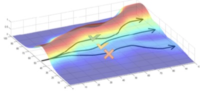
Trajectories that climb toward higher reward get reinforced; ones that don't, don't. Source: Stanford CS224R. Concretely, suppose a trajectory gets . Then
is a large update, and the actions in that trajectory become more likely. If instead , there’s almost no update. If , the update flips direction entirely: the policy learns “avoid doing what I just did.” ↩
-
Plain Monte Carlo only estimates expectations. If you sample trajectories , averaging computes
not . The first expression, , is not an expectation, since there’s no multiplying the integrand. If you ran the policy and averaged over the sampled trajectories, the law of large numbers says you’d be estimating
a different integral, not the one we want. Short of that, the only way to compute exactly is brute force: enumerate every possible trajectory, which is infeasible since there are enormously many of them, often effectively infinite.
After the log-derivative trick, using , the integral becomes
which now is an expectation:
↩ -
Suppose we collect 3 episodes:
Episode Return 1 10 2 2 5 1 3 20 3 Each episode’s contribution is :
Averaging over the 3 episodes:
which gives the update . ↩
-
Step 3 is just the ordinary neural-network parameter update, with a plus sign because we are ascending instead of descending a loss. In standard supervised training the update is
where stands for all trainable parameters at once. If the network is , that one line means
with every trainable parameter moving along its own gradient. Policy gradient uses exactly the same rule, ; the only special part is how the loss is defined, (see the surrogate objective below), and minimizing that loss is the same thing as ascending . So the pipeline is: RL supplies the objective, backprop computes the gradients, and a standard optimizer updates the network’s parameters. ↩
-
Take the same 3 episodes, but suppose episode 3 happened to get a lucky return of instead of :
Episode Return 1 10 2 20 2 5 1 5 3 1000 3 3000 The average becomes , almost entirely determined by episode 3. Resample a different batch of 3 episodes without that lucky outlier, and the estimate could be back down near , even though the policy hasn’t changed at all. That swing between batches, driven by which episodes happened to be sampled, is the high variance. ↩
-
Imagine a robot walking:
Time Action Reward step forward step forward step forward big step backward step forward Total reward: .
Under the original REINFORCE estimator, every action gets multiplied by this same total return, : is scaled by , and so is , and so on for every timestep:
Even the three good forward steps get blamed: they didn’t cause the backward mistake at , yet REINFORCE blames the entire trajectory for it. ↩
-
Using the same rewards (), the reward-to-go estimator gives each action its own future return, :
Now each action gets a learning signal that reflects its actual consequences. In particular, : the last forward step, which happened entirely after the mistake, correctly gets a positive signal instead of sharing in the blame. The resulting gradient estimate is
each action weighted by its own instead of the same flat . ↩
-
Suppose we run 3 trajectories:
Trajectory Reward 100 110 105 Average reward: . All three trajectories get a positive update, even , which is actually the worst trajectory of the batch: REINFORCE just sees “reward , increase probability,” without accounting for the fact that is below average. ↩
-
With : trajectory 1 gets , a negative signal, reduce its probability. Trajectory 2 gets , a positive signal, increase it. Trajectory 3 gets , no update, exactly average behavior. This is a much more informative learning signal than the raw rewards. ↩
-
Suppose a batch of rewards is . Without a baseline, the gradient is scaled by these large, similar numbers, so its magnitude fluctuates with whatever the rewards happen to be. Subtracting the average () gives : much smaller numbers, centered at zero, with below-average trajectories now correctly getting a negative signal. ↩
-
Consider training a robot policy to fold a jacket, with reward given only at the end of the episode: for a neatly folded jacket, for an okay job with some wrinkles, for failing to fold it at all. Suppose 4 trajectories:
Trajectory Outcome Reward Doesn’t touch the jacket Folds only the sleeves Flattens the jacket but doesn’t fold it Folds it perfectly The baseline is , and each trajectory’s weight is :
and get the exact same weight, , even though flattening the jacket () is a real step toward folding it, while never touching it () makes no progress at all. Because the reward only arrives at the end, the baseline has no way to tell these two failures apart. ↩
-
Suppose trajectories, each with steps. There are terms in the sum. Calling
backward()separately for each one would mean 100,000 backward passes, one per state-action pair, far too slow to be practical. ↩ -
isn’t a meaningful loss value on its own the way a supervised loss is, where a lower number means a better fit. Its only job is to make
loss.backward()produce the correct gradient; the number itself isn’t something worth tracking for its own sake. ↩ -
Writing out the full ratio before canceling anything,
the initial state distribution and the environment dynamics appear identically in the numerator and denominator, so they cancel:
the initial state distribution (blue) and the transition dynamics (orange) drop out entirely, leaving only the ratio of policy probabilities at each timestep. ↩
-
Suppose a single-step decision between two actions, and the old and new policies assign:
Action (old) (new) Left 0.8 0.4 Right 0.2 0.6 If the trajectory we collected took Right, its importance weight is : this trajectory becomes three times as important, since the new policy likes Right much more than the old one did. If instead the trajectory had taken Left, : it becomes half as important, since the new policy likes Left less than the old one did. This is exactly how old data gets corrected for the policy having changed. ↩
-
Suppose every one of the per-timestep ratios happens to be a modest (the new policy is just slightly more likely to take each action than the old one). Over steps, the product is , a huge multiplier. If instead every ratio is , the product is , close to zero. A slight, consistent per-step difference between the two policies compounds multiplicatively over a long trajectory, which is why this off-policy estimator tends to be very high variance in practice. ↩
-
This is similar in spirit to the move from the trajectory’s return to the reward-to-go earlier in this note: both replace one trajectory-wide quantity with a separate quantity per timestep. There, the motivation was credit assignment, an action shouldn’t be weighted by rewards it couldn’t have influenced. Here, the motivation is variance reduction, an action shouldn’t be reweighted by a product of every ratio in the trajectory, only its own. Same move, different reason. ↩
-
Suppose the old and new policies choose between two actions:
Action (old) (new) Left 0.51 0.55 Right 0.49 0.45 These policies behave almost identically, so trajectories collected under are still representative of what would experience. Compare a case where the policies diverge sharply instead:
Action (old) (new) Left 0.99 0.01 Right 0.01 0.99 Here the old data is almost entirely “Left” trajectories, but the new policy almost always chooses “Right.” The old dataset no longer describes what the new policy actually does. ↩
-
Suppose always explores the left side of a maze (start → left corridor → treasure), while always goes right (start → right corridor → monster). The old dataset has zero experience with the right corridor, so there’s no way to estimate what would actually earn there: the data needed to make that estimate was never collected. ↩