Instruction and Supervised Finetuning
July 6, 2026 · Updated August 31, 2026
Contents
Instruction tuning is the next step after pre-training and the foundation of post-training. It teaches the model how humans want it to respond.
Instruction tuning uses the same loss function as pretraining (cross-entropy next-token prediction), but the way we train is quite different.
During training, the model is usually only predicting the completion. It is not trying to predict the prompt.
The data is different too. Instead of raw internet text, we have data in this format:
<User>
What is the capital of France?

<Assistant>
Paris.
and we only compute loss on the assistant tokens. The prompt is treated as context.
Loss masking
Take the example “User: 2+2? Assistant: 4”. After tokenization, imagine it becomes
The dataloader creates
Input  = tokens[:-1]
Target = tokens[1:]
and a loss mask:
User tokens      → 0
Assistant tokens → 1
Step 1: shift the sequence. The model input is and the targets are . Internally the model predicts:
| Position | Context | Predicts |
|---|---|---|
| 1 | User: | 2+2? |
| 2 | User: 2+2? | Assistant: |
| 3 | User: 2+2? Assistant: | 4 |
| 4 | User: 2+2? Assistant: 4 | <EOS> |
Normally (pretraining), we’d compute
or, more compactly,
Every prediction contributes.
Instruction tuning adds a mask :
| Prediction | Mask |
|---|---|
| predict 2+2? | 0 |
| predict Assistant: | 0 |
| predict 4 | 1 |
predict <EOS> | 1 |
The loss becomes
Substituting the mask,
which simplifies to
The model still computes the probability distributions for predicting “2+2?” and “Assistant:”; those forward passes happen anyway because the Transformer processes the whole sequence. But since their mask is 0, they contribute nothing to the loss, so no gradient comes from those predictions.
”If we’re going to ignore the prompt tokens, why predict them at all?”
For the sequence
User: What is 2+2?
Assistant: 4
after tokenization:
x₁ = User:
x₂ = What
x₃ = is
x₄ = 2+2?
x₅ = Assistant:
x₆ = 4
x₇ = <EOS>
The Transformer receives . Because of the causal mask, every position independently computes its hidden state:
Then every hidden state goes through the same output layer:
So the model naturally produces six predictions simultaneously. In principle, we could have skipped the first five: you could imagine writing code like
for t in assistant_positions:
    compute_logits(h_t)
But that’s not how Transformer implementations are designed, for two reasons.
1. The GPU is extremely efficient at doing one large matrix multiplication. Computing for all positions at once is a single big matmul; looping over selected positions is slower than computing everything and masking the loss.
2. Even though we ignore their losses, we still need their hidden representations. Every token is first converted into an embedding vector:
The hidden state at the “Assistant:” position is computed from all of them:
Suppose attention assigns these weights to the previous tokens:
| Previous token | Attention weight |
|---|---|
| User: | 0.02 |
| What | 0.08 |
| is | 0.10 |
| 2+2? | 0.75 |
| Assistant: | 0.05 |
So the hidden representation becomes roughly
The model predicts “4” using only :
If , the loss is .
During backpropagation we compute . Since depends on all the earlier embeddings, the chain rule tells us
and similarly for , , . So even though the prompt predictions contribute no loss terms of their own, the prompt tokens’ representations still receive gradients; they are updated as context for the assistant tokens.
The same holds layer by layer. Suppose we start with embeddings . At layer 1, the model computes new hidden states , where attends to . Layer 2 does not use the embeddings anymore; it computes by attending to . So the hidden states at the prompt positions have to be computed at every layer; later layers depend on them.
Principles
-
With instruction tuning, small focused datasets can achieve strong performance and high quality data is key.
-
Pretraining already teaches the model core concepts. Instruction tuning mainly teaches how to respond. Eg: 1M diverse high quality prompts is enough, no need for say 100M. Eventually we’re repeating similar situations and the model has already learned the behavior.
-
Prompts in the dataset should be of similar distribution as intended usage. Eg: If the model will be used mainly for coding, train it on coding instructions; if it will be used for customer support, train it on support-style conversations.
-
It is fine if the dataset has some imperfect examples as the noise can be corrected during the RLHF step.
Batch size
Instruction tuning can use smaller batches than pretraining. The pretraining dataset is incredibly enormous and consists of diverse domains. The gradients from any one document are noisy. Large batches help average out this noise. In instruction tuning on the other hand, examples come from a narrower distribution. The gradients from different examples are already much more similar, so we don’t need as much averaging.
During pretraining we might take 1024 packed1 rows (for 7B) or 2048 packed rows (for 13B), whereas 256 prompts for instruction tuning.
Using smaller batches means fewer GPUs. If each GPU can process 16 examples and batch size is 2048, then 2048 / 16 = 128 GPUs. With SFT suppose batch size = 256, then 256 / 16 = 16 GPUs. If we keep using 128 GPUs, that’s 2 examples per GPU; communication between GPUs would dominate the computation, making training inefficient. Distributed training frameworks also have practical minimum batch sizes per device for stable, efficient execution.
Practitioners also train the same instruction tuning setup over multiple training seeds for randomness in training (dropout, data shuffling) and keep the best checkpoint instead of spending all their compute on a single run.
Learning rate
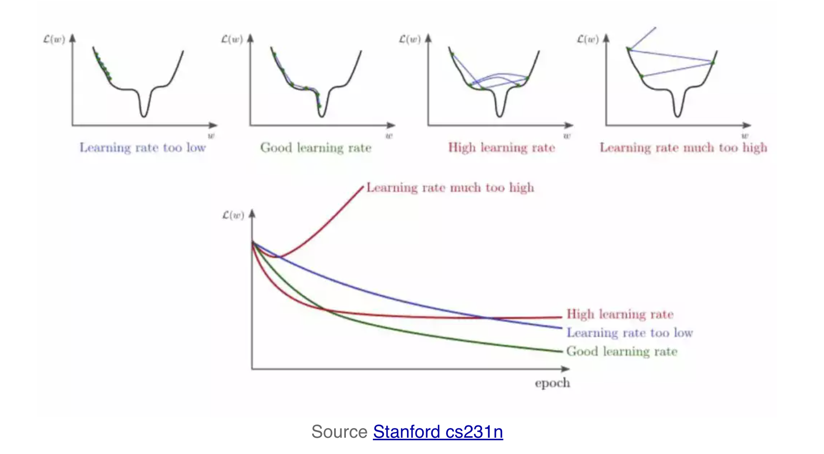
The learning rate used in instruction tuning is one to two orders of magnitude smaller than pretraining. The gradient tells what direction to move in, and the learning rate decides how far we move.
where = model weights, = gradient, = learning rate.
A learning rate that is too high can cause the model to overfit the training data. A learning rate that is too low can cause the model to underfit the training data. Pretraining can use a large learning rate as it starts with random weights and knows nothing; large updates help it learn quickly. With SFT the model already has domain knowledge. Instruction tuning wants to teach small behavioural changes without rewriting things the model already knows, and benefits from tiny adjustments. Another reason is that since the batch size with SFT is smaller, the batch gradient estimates could be noisier, which makes taking large steps risky.
OLMo 2 learning rate example:
- Pretraining:
- Instruction tuning:
OLMo 3 uses a higher SFT learning rate of , because its training infrastructure uses sequence packing, which fits multiple examples into each training sequence and increases the effective batch size measured in useful tokens. Eg: without packing, 5,000 useful tokens; with packing, 25,000 useful tokens. This makes the gradient estimate much more accurate.
Linear scaling rule: If you increase the batch size by , you can often increase the learning rate by about as well while maintaining similar optimization behavior. This is because bigger batches produce less noisy gradients, which means larger steps can be taken without overshooting.
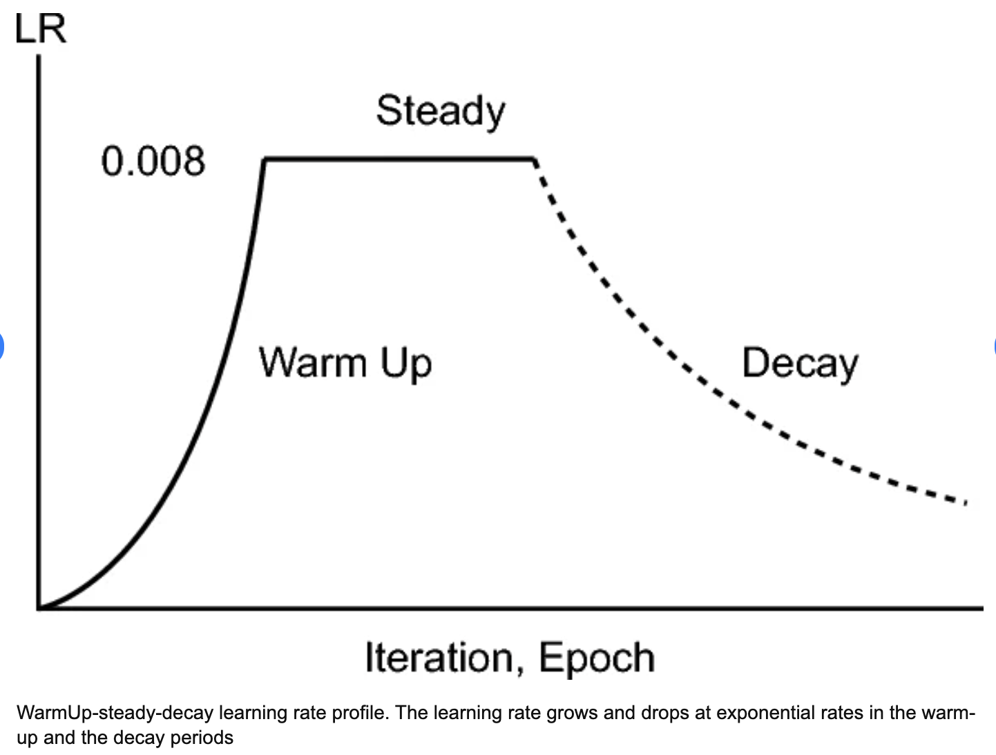
A learning rate warmup is usually performed, where the learning rate initially starts smaller and then increases: early in training, gradients can be unstable because the optimizer’s internal statistics (e.g., in AdamW) are not yet well adapted. Starting with a tiny learning rate avoids making an overly aggressive first update.
Experiment: Learning rate sweep
To make the “one to two orders of magnitude below pretraining” guidance concrete, I fine-tuned allenai/OLMo-2-0425-1B (base, no chat template, borrowed one from allenai/OLMo-2-0425-1B-SFT) on HuggingFaceH4/no_robots (~9.5K conversations) for 3 epochs at bf16, batch size 4 × 8 gradient accumulation steps (effective batch 32), at , holding everything else fixed (10% linear warmup, weight decay 0, grad clip 1.0). Padding: batch length is dynamic, not fixed: each batch is padded to whichever of its 4 examples is longest, using the tokenizer’s <|pad|> token. E.g. a batch with example lengths 26, 60, 15, 40 gets padded to 60: the 26-token example receives 34 <|pad|> tokens, the 15-token one receives 45, etc. Padded positions get attention_mask = 0 (invisible to attention) and label = -1002 (masked, same as prompt tokens), so padding never contributes to the loss.
Final loss (after 3 epochs):
| lr | final loss |
|---|---|
| 1e-6 | 2.1055 |
| 5e-6 | 2.0469 |
| 5e-5 | 1.7295 |
Sample generations near the end of training (eval prompt: “What is the capital of France?”):
| lr | output |
|---|---|
| 1e-6 | <|user|><|assistant|><|user|><|assistant|>...: degenerate repetition; never learned to answer |
| 5e-6 | The capital of France is Paris.<|endoftext|>: clean, correct, stops |
| 5e-5 | Paris is the capital of France. It is also the country's most populous city and is located on the river Seine. The city has a population of 2.2 million...: correct and stops, but pads with unrequested detail |
Lowest loss does not mean best behavior: 5e-5 fits the training distribution’s style fastest (hence lowest loss) but shows the first signs of overfitting: earlier checkpoints (steps 100-200) at this lr produced confidently wrong padding (e.g. claiming Paris was “founded in 753 BC,” the traditional founding date of Rome). 1e-6 never escapes base-model continuation behavior within the step budget; too low to converge. 5e-6 is the sweet spot in this sweep: it answers and stops cleanly without the padding/hallucination artifacts of the higher lr.
TODO
These notes were made reading the RLHF book, watching the videos, and having a spirited discussion with ChatGPT.
Footnotes
-
This is a very common optimization. Suppose your model accepts sequences of length 4096 tokens and you have three documents: Doc A (500 tokens), Doc B (700 tokens), Doc C (600 tokens). If you trained them separately (Row 1: 500 useful, 3596 padding; Row 2: 700 useful, 3396 padding; Row 3: 600 useful, 3496 padding), most computation is wasted. Instead, multiple documents are concatenated into one long sequence: 4096 tokens = Doc A + Doc B + Doc C + Doc D + … until the row is full. This is called packing. Packing is not used in instruction tuning: unlike during pretraining, we don’t want to concatenate unrelated conversations, as each prompt–answer pair is a separate example. ↩
-
-100 isn’t special mathematically; it’s just PyTorch’s chosen sentinel value.
F.cross_entropy(..., ignore_index=-100): theignore_indexargument intorch.nn.functional.cross_entropy(andnn.CrossEntropyLoss) tells PyTorch: “if a label equals this value, skip it entirely, don’t include it in the loss, don’t compute a gradient from it.” ↩