← All notes

Negative Log-Likelihood, Entropy, Cross-Entropy, and KL Divergence

September 12, 2026 · Updated September 24, 2026

Throughout this note, let $z$ be an outcome, such as a class, token, or complete sequence, and let $p$ and $q$ be probability distributions over the same outcomes.

Negative Log-Likelihood

Suppose an observed outcome is $z$ and a model assigns it probability $q(z)$. Its likelihood is $q(z)$, so its negative log-likelihood (NLL) is

A likely outcome has a small NLL, while an outcome assigned near-zero probability has a very large NLL. For a dataset of $N$ observed outcomes $z_1,\ldots,z_N$, the average loss is

When the observations are drawn from a distribution $p$, the expected NLL under $p$ is the cross-entropy $H(p,q)$ defined below.

Entropy

In information theory, entropy ($H$) measures the average uncertainty, surprise, or information content in a distribution of messages or data. The concept was introduced by Claude Shannon.

For a distribution $p$, entropy is

For example:

• A concentrated distribution such as $(0.99,0.01)$ has low entropy.
• A flat distribution such as $(0.5,0.5)$ has high entropy.

Equivalently, entropy is the expected surprise when outcomes come from $p$ and are evaluated using $p$ itself:

Cross-Entropy

Cross-entropy measures how well a distribution $q$ predicts outcomes distributed according to a target distribution $p$:

This form comes from expected negative log-likelihood. For one outcome $z$, the loss under $q$ is $-\log q(z)$. Because $p$ produces that outcome with probability $p(z)$, averaging the loss over outcomes from $p$ gives

Here, $p(z)$ determines how much weight the target distribution gives outcome $z$, while $-\log q(z)$ measures how poorly $q$ predicts it.

KL Divergence

KL divergence measures how one probability distribution differs from another. For discrete distributions, it is¹

For continuous distributions with densities $p(z)$ and $q(z)$, the sum becomes an integral:

KL divergence can also be written as an expectation. When $p$ is the target distribution and $q$ is the approximation, the direction from $p$ to $q$ is called forward KL:

Swapping the arguments gives the reverse KL:

The direction changes the distribution used to weight the expectation: forward KL samples from $p$, while reverse KL samples from $q$. KL divergence is not symmetric, so the order of the arguments matters:

By Gibbs’ inequality, both directions are nonnegative. The individual log-ratio terms inside the expectation can still be negative.²

Cross-Entropy and Forward KL

Cross-entropy decomposes into the entropy of the target distribution and the forward KL divergence:

When $p$ is fixed, $H(p)$ is constant. A learned distribution $q$ can therefore minimize cross-entropy only by minimizing forward KL:

Both objectives consequently have the same optimum.³ This is why a cross-entropy objective against a fixed teacher or data distribution can be interpreted as forward-KL minimization.

SFT and RL Through the KL Lens

Adapted from Cameron R. Wolfe’s explanation of SFT and RL through KL divergence.[2]

The same KL perspective clarifies an important difference between supervised fine-tuning (SFT) and KL-regularized reinforcement learning. For a fixed prompt $s$, let $u$ denote a complete output sequence. To keep the equations uncluttered, all distributions below are implicitly conditioned on $s$.

The key distinction is the distribution from which completions are sampled. SFT averages its loss over a fixed dataset distribution, so its training signal is offline. RL averages reward over completions sampled from the current model, so its training signal is online, or on-policy.

SFT as Forward KL

Let $p_{\mathrm{data}}$ be the distribution represented by the SFT dataset and $q_\theta$ the model being trained. The SFT negative log-likelihood is

Because $H(p_{\mathrm{data}})$ does not depend on the model parameters, minimizing the SFT loss is equivalent to minimizing the forward KL divergence:

The data distribution appears first in the KL and therefore supplies the samples in the expectation.

KL-Regularized RL as Reverse KL

For KL-regularized RL, let $q_\theta$ be the current policy, $q_{\mathrm{ref}}$ a fixed reference policy, $r(u)$ the reward, and $\beta>0$ the strength of the KL penalty. The idealized objective is

Define the reward-induced target distribution

This target reweights the reference policy toward higher-reward completions. Substituting its log-probability into the reverse KL gives

Because $Z$ does not depend on $\theta$, maximizing this KL-regularized RL objective is equivalent to minimizing $D_{\mathrm{KL}}(q_\theta\parallel p_R^*)$. This is a reverse KL because the learned policy appears first and the fixed reward-induced target appears second.

The explicit term $D_{\mathrm{KL}}(q_\theta\parallel q_{\mathrm{ref}})$ inside $J_{\mathrm{RL}}$ is the regularizer that keeps the policy near the reference. The reverse-KL interpretation comes from rewriting the complete reward-plus-regularization objective.

Mode Covering Versus Mode Seeking

These two KL directions help explain the different tendencies of SFT and RL:

• SFT is mode-covering. Forward KL averages over $u\sim p_{\mathrm{data}}$. If the data assigns positive probability to a completion while the model assigns it near-zero probability, its contribution $-p_{\mathrm{data}}(u)\log q_\theta(u)$ grows without bound. The model is therefore encouraged to assign probability across all modes represented in the data.
• KL-regularized RL is mode-seeking. Reverse KL averages over $u\sim q_\theta$. Completions to which the current policy assigns very little probability are rarely sampled and receive little direct weight. The policy can therefore concentrate on a subset of high-reward modes instead of covering every mode of $p_R^*$.

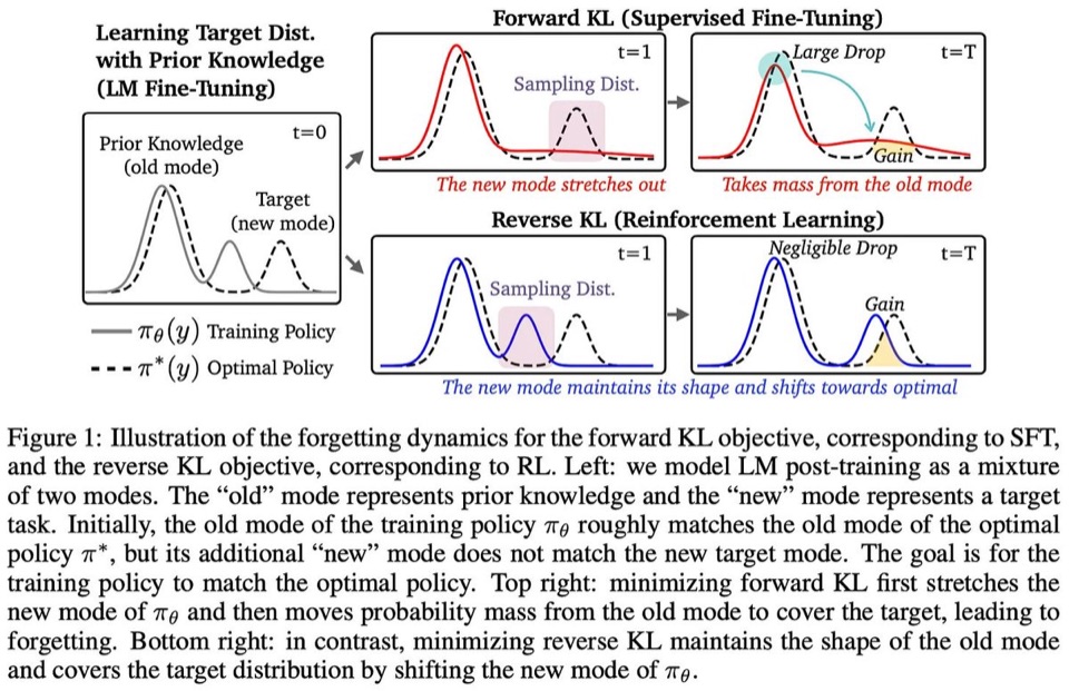
Mode covering and mode seeking describe tendencies, not guarantees. The practical behavior also depends on model capacity, optimization, reward quality, sampling, and the strength $\beta$ of the reference-policy constraint.

TODO

• Jensen-Shannon divergence

Bibliography

- Howard Chen, Noam Razin, Karthik Narasimhan, and Danqi Chen, “Retaining by Doing: The Role of On-Policy Data in Mitigating Forgetting,” arXiv preprint arXiv:2510.18874, 2025.
- Cameron R. Wolfe, “SFT and RL Training Objectives as Forward and Reverse KL Divergence,” X, 2026.