Knowledge Distillation for Language Models

August 29, 2026 · Updated October 6, 2026

Contents

Foundations

Adapted from “Everything You Need to Know about Knowledge Distillation”.

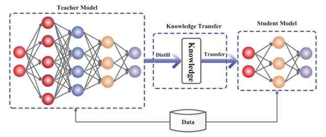
Knowledge distillation transfers knowledge from a large model, called the teacher, to a smaller model, called the student. It allows a smaller, faster model to inherit much of the teacher’s capability without having to learn solely from the original hard labels, making powerful models cheaper and easier to deploy.[1]

Instead of training the student only on correct answers, we train it on the teacher’s full probability distribution over possible outputs. This tells the student not only which answer the teacher prefers, but also how confident the teacher is about each alternative.

This helps because the teacher’s full probability distribution carries far more information than a single correct answer. Those probabilities carry information about how the larger model thinks: which alternatives it considers and how confident it is in each one. For an image of a dog, a teacher might output dog: 0.9, wolf: 0.08, cat: 0.001. The relative probabilities reveal that the teacher considers dogs more similar to wolves than to cats. Hinton called this hidden similarity structure dark knowledge, and it is exactly the kind of signal a small model struggles to learn from hard labels alone.[12]

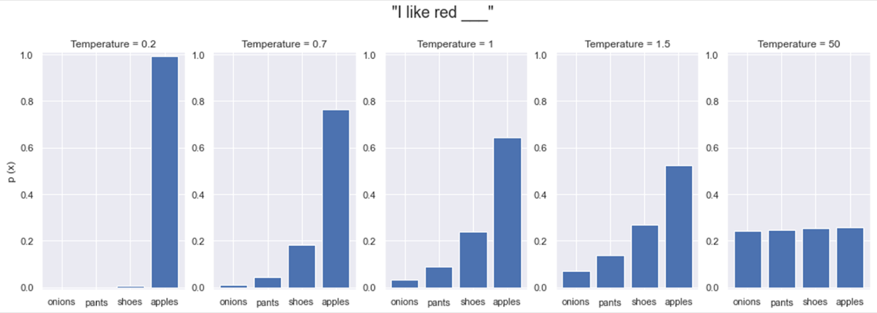
A large teacher model transfers knowledge learned from shared data to a smaller student model. — Teacher-to-student knowledge transfer. Image credit: Gou et al., “Knowledge Distillation: A Survey” [1].

Softmax is a mathematical function that converts raw scores, called logits, into probabilities. It helps a model express its relative confidence that an input belongs to each category, or class, while ensuring that the output values sum to 1.¹

A temperature parameter $T$ can be added to softmax to control how sharp or flat its probability distribution is. At $T=1$ , it behaves as ordinary softmax. Lower temperatures ( $T<1$ ) sharpen the distribution, making high-logit options more dominant; higher temperatures ( $T>1$ ) flatten it, spreading probability mass across more options.[2]

In knowledge distillation, the one-hot ground-truth labels are hard targets, while the teacher’s probability distribution, often softened with $T>1$ , provides soft targets. The softer distribution reveals which alternatives the teacher considers similar or plausible, giving the student more information than the correct label alone.[1]

Five bar charts show the probability of the words onions, pants, shoes, and apples completing the sentence I like red at temperatures 0.2, 0.7, 1, 1.5, and 50. The distribution changes from almost entirely apples at low temperature to nearly uniform at high temperature. — Increasing temperature flattens the distribution over candidate words. Source: Hopsworks, “LLM Temperature” [2].

Training with soft targets

Soft targets are commonly used for distillation training. A typical procedure has three steps:

Train the teacher model on the original task and dataset.
Run the training examples through the teacher to produce logits. Convert these logits into soft targets using softmax with a higher temperature, which makes the probability distribution softer.
Train the student on the soft targets, often alongside the hard targets (the ground-truth labels). The objective combines a distillation loss that measures the difference between the student’s and teacher’s output distributions with a standard supervised loss on the hard targets.

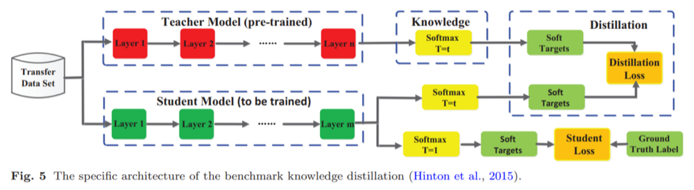
A pretrained teacher and a student process a transfer dataset. Temperature-scaled softmax produces soft targets for both models, a distillation loss compares them, and a separate student loss compares the student's ordinary softmax output with the ground-truth label. — The benchmark knowledge-distillation training pipeline combines a distillation loss on softened outputs with a supervised loss on ground-truth labels. Source: Gou et al., “Knowledge Distillation: A Survey” [1], Figure 5.

Through this process, the student learns not only which answer is correct, but also the teacher’s relative confidence across alternatives. Probability assigned to incorrect categories can encode similarities that hard labels discard, giving the student a richer training signal and helping it imitate the teacher’s behavior. By optimizing a weighted combination of the supervised and distillation losses, a student can approach the teacher’s accuracy despite having far fewer parameters.[1]

Types of knowledge distillation

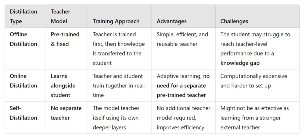
There are three main ways to transfer knowledge during training: offline distillation, online distillation, and self-distillation.

A table comparing offline, online, and self-distillation by teacher model, training approach, advantages, and challenges. Offline distillation uses a fixed pretrained teacher, online distillation trains teacher and student together, and self-distillation uses the model itself as the teacher. — Offline, online, and self-distillation differ in where the teacher signal comes from and when the teacher is trained. Source: Ksenia Se and Alyona Vert, “Everything You Need to Know about Knowledge Distillation”.

Distillation loss

The loss proposed by Hinton, Vinyals, and Dean is a weighted combination of two cross-entropy objectives: one makes the student imitate the teacher, and the other makes it predict the true label.[3]

Let $v_i$ be the teacher’s logit and $z_i$ the student’s logit for class $i$ . At temperature $T$ , their probability distributions are

p_i^{(T)} = \frac{e^{v_i/T}}{\sum_j e^{v_j/T}}, \qquad q_i^{(T)} = \frac{e^{z_i/T}}{\sum_j e^{z_j/T}}.

The distillation loss is the cross-entropy between the teacher’s and student’s softened distributions:

\mathcal{L}_{\text{soft}} = -\sum_i p_i^{(T)} \log q_i^{(T)}.

Because the teacher distribution is fixed, this cross-entropy objective can equivalently be viewed as minimizing $D_{\mathrm{KL}}\!\left(p^{(T)} \parallel q^{(T)}\right)$ , as shown in Cross-Entropy and Forward KL. The hard-target loss is ordinary cross-entropy between the one-hot true label $y$ and the student’s temperature- $1$ distribution:

\mathcal{L}_{\text{hard}} = -\sum_i y_i \log q_i^{(1)}.

Using $\alpha$ and $\beta$ for the two loss weights, the complete objective can be written as²

\mathcal{L} = \alpha T^2 \mathcal{L}_{\text{soft}} + \beta \mathcal{L}_{\text{hard}}.

Both terms use the same student logits. The soft term evaluates them at the same high temperature used by the teacher, while the hard term evaluates them at $T=1$ . The paper does not prescribe universal values for $\alpha$ and $\beta$ , although it reports generally placing considerably less weight on the hard-target term. In its speech-recognition experiments, it used a relative hard-target cross-entropy weight of $0.5$ .[3] Here, the $T^2$ factor is present because, when the soft- and hard-target losses are combined, increasing $T$ would otherwise make the soft-target gradient weaker relative to the hard-target gradient.[3]

Adapting distillation to language models

Adapted from “Adapting Knowledge Distillation for LMs”.

Token-level distillation

Knowledge distillation is not limited to language modeling. In a multiclass classification problem, it usually matches one output distribution for each input. An autoregressive language model instead predicts a distribution at every sequence position, so the distillation objective can be decomposed into a sum of per-token distribution-matching losses.

Let $s$ be the source sentence or prompt, $u=(u_1,\ldots,u_J)$ a complete output sequence produced by the teacher, and $\mathcal{V}$ the model’s tokenizer vocabulary. Continuing the notation above, let $p$ be the teacher’s next-token distribution and $q$ the student’s next-token distribution. The prefix $u_{<j}=(u_1,\ldots,u_{j-1})$ contains the tokens preceding position $j$ .

Kim and Rush originally formulated this objective as word-level distillation for neural machine translation. Because their setup used a word vocabulary, the same expression is better read for modern language models as per-token distribution matching over the tokenizer vocabulary:[4]

\mathcal{L}_{\text{token-KD}} = -\sum_{j=1}^{J}\sum_{k=1}^{|\mathcal{V}|} p\!\left(u_j=k \mid s,u_{<j}\right) \log q\!\left(u_j=k \mid s,u_{<j}\right).

In this offline formulation, the loss is generally computed over a static text sequence already included in the training corpus. It has the ordinary cross-entropy form. At each position $j$ , the teacher distribution $p(\cdot \mid s,u_{<j})$ assigns probability to every possible next token $k\in\mathcal{V}$ , and the student is penalized when its distribution $q(\cdot \mid s,u_{<j})$ puts too little probability on tokens the teacher considers likely. The inner sum aggregates this mismatch across the vocabulary, while the outer sum adds the loss across the complete sequence.³

Sequence-level distillation

Sequence-level distillation instead treats $\mathcal{U}$ as the space of all possible output sequences and asks the student to match the teacher’s distribution over complete sequences. The exact objective requires summing over every $u\in\mathcal{U}$ , an exponentially large space. Kim and Rush make this tractable by approximating the teacher distribution with a point mass on one high-probability teacher output $\hat{u}$ found using beam search:[4]

\hat{u} = \operatorname{BeamSearch}_{p}(s) \approx \arg\max_{u\in\mathcal{U}} p(u\mid s).

Under this approximation, the sequence-level cross-entropy reduces to the negative log-probability that the student assigns to $\hat{u}$ :⁴

\begin{aligned} \mathcal{L}_{\text{seq-KD}}(s) &= -\sum_{u\in\mathcal{U}} p(u\mid s)\log q(u\mid s) \\ &\approx -\log q(\hat{u}\mid s) \\ &= -\sum_{j=1}^{|\hat{u}|} \log q\!\left(\hat{u}_j \mid s,\hat{u}_{<j}\right). \end{aligned}

Sequence-level KD moves toward modern distillation methods because the teacher now generates the tokens that supervise the student. However, the teacher outputs are generated a priori, stored, and then treated as a fixed training corpus. We will refer to this setup as offline KD. Replacing the intractable distribution over all possible sequences with fixed teacher generations makes training practical and sets up the later contrast with on-policy distillation, where the training sequences change as the student changes.

The token- and sequence-level objectives above are cross-entropies between a fixed teacher distribution and the student. As explained in Cross-Entropy and Forward KL, minimizing either objective is therefore equivalent to minimizing forward KL from the teacher to the student.

Their fixed teacher-generated training corpora also place them on the offline side of the sampling distinction between SFT and RL. On-policy distillation will instead train on completions sampled from the current student.

Distillation in practice

Adapted from Julia Turc, “Knowledge Distillation: How LLMs train each other”.

Not all distillation claims are created equal. In the open-weight ecosystem, Google distilled its Gemini models into Gemma 2 and Gemma 3, while Meta distilled Llama 4 Behemoth into Llama 4 Scout and Maverick. DeepSeek-R1 follows a different pattern: its mixture-of-experts teacher generated reasoning data used to fine-tune dense students from other model families, namely Llama 3.1 and Qwen 2.5.

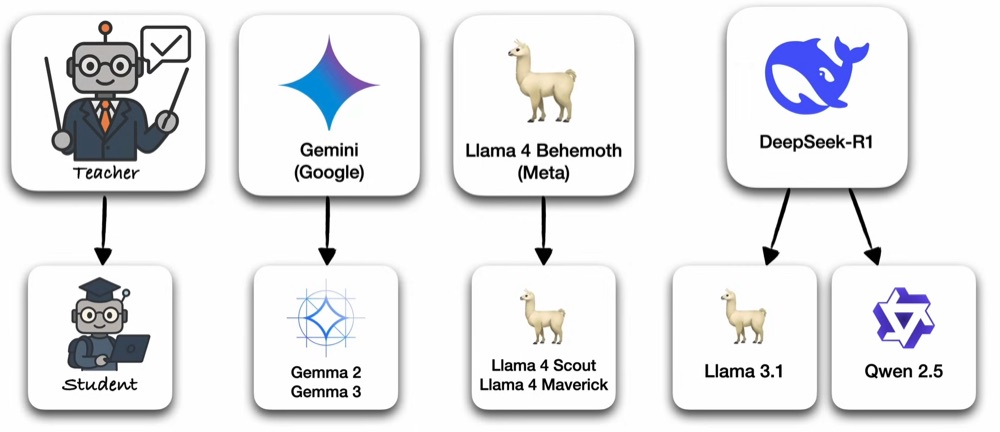
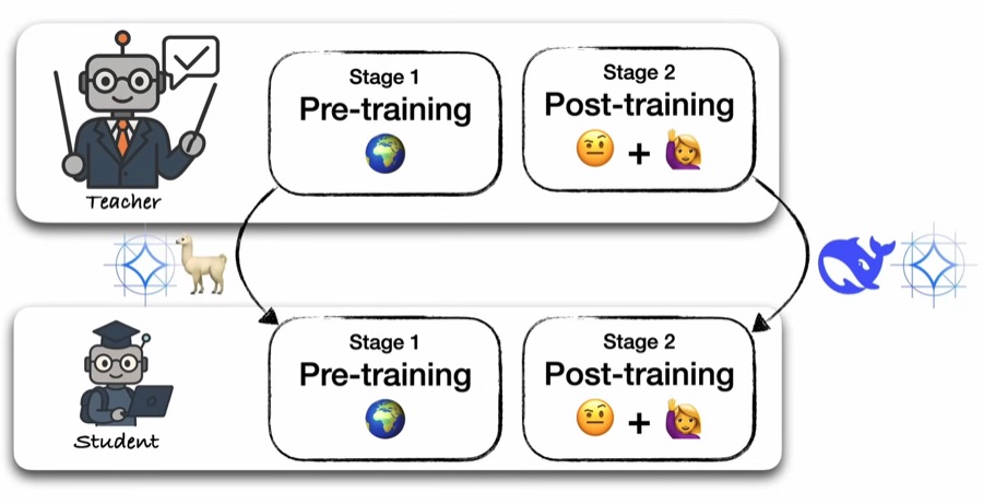
A comparison of teacher-to-student distillation, including Gemini to Gemma 2 and Gemma 3, Llama 4 Behemoth to Llama 4 Scout and Maverick, and DeepSeek-R1 to Llama 3.1 and Qwen 2.5. — Examples of how knowledge distillation is used across open-weight model families. Source: Julia Turc, “Knowledge Distillation: How LLMs train each other” [8].

Distillation can be applied at two main stages of the LLM training pipeline, or at both:

Pre-training. The model learns from an enormous corpus, much of it gathered from the web, through next-token prediction. Meta used codistillation from Llama 4 Behemoth during Llama 4 Maverick’s pre-training.[5]
Post-training. The pretrained model is fine-tuned on instruction-response pairs to align its behavior with human preferences and strengthen abilities such as reasoning. DeepSeek used this stage to train dense Llama 3.1 and Qwen 2.5 students on reasoning data generated by DeepSeek-R1.[6]
Both stages. Gemma 3 used distillation during pre-training and again during post-training.[7]

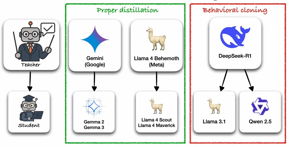
A teacher and student training pipeline showing that knowledge distillation can be applied during pre-training, post-training, or both stages. — Distillation can transfer teacher knowledge during pre-training, post-training, or both. Source: Julia Turc, “Knowledge Distillation: How LLMs train each other” [8].

Proper distillation and behavioral cloning

However, the exact transfer mechanism differs across model families. Google and Meta use logit-level distillation, which the source calls proper distillation. A more precise name for DeepSeek-R1’s approach is behavioral cloning: its students imitate teacher-generated sequences rather than matching the teacher’s full token probability distribution.[8]

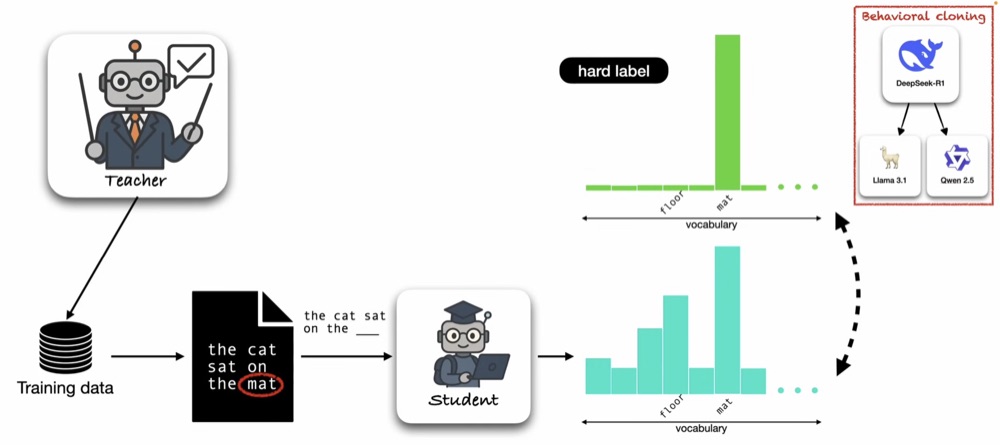
Gemini-to-Gemma and Llama 4 Behemoth-to-Scout and Maverick are grouped under proper distillation, while DeepSeek-R1-to-Llama 3.1 and Qwen 2.5 is grouped under behavioral cloning. — Logit-level distillation transfers full probability distributions, while behavioral cloning trains on teacher-generated sequences. Source: Julia Turc, “Knowledge Distillation: How LLMs train each other” [8].

In the case of proper distillation, assume the teacher is already trained and fixed while the student is being trained. One update proceeds as follows:

Sample a document from the training corpus and train the student to predict it one token at a time. Suppose the document is the cat sat on the mat, and at position 6 the target token is mat.
Feed the incomplete prefix, the cat sat on the, to both the teacher and the student.
Both models output a probability distribution over the entire vocabulary. The teacher’s distribution becomes the student’s soft label.
Update the student’s weights to minimize the gap between its prediction and the teacher’s distribution using the soft-target distillation loss. In the combined objective described above, this can be paired with a separate hard-target loss on the one-hot corpus token, which is mat in this example.

At each token position, the student learns to match the teacher's complete vocabulary distribution. Source: Julia Turc, “Knowledge Distillation: How LLMs train each other” [8].

In DeepSeek-R1’s behavior-cloning-style distillation, the input prompts may be collected in advance, but the teacher generates the target completions. The student is then trained on those completions using ordinary next-token prediction.[6]

The crucial difference is that the labels are no longer soft. At each position, the target is one-hot: if the generated next token is mat, then mat receives 100% of the target probability mass and every other token receives 0%. The student therefore learns to imitate the teacher’s realized outputs. It can copy any written reasoning trace in those outputs, but it does not receive the teacher’s full probability distribution over alternative tokens or its hidden internal computation.

Behavioral cloning pipeline in which a teacher generates training data, then a student predicts the next token from an incomplete sequence using a one-hot hard label that assigns all target probability to the token mat. — Behavioral cloning trains the student on the teacher's sampled tokens as hard labels rather than on its full vocabulary distribution. Source: Julia Turc, “Knowledge Distillation: How LLMs train each other” [8].

Why not use proper distillation everywhere?

Proper distillation gives the student a richer target than behavioral cloning, but it is not always practical for two reasons:

Teacher access. Distillation requires access to the teacher’s logits, making it a white-box method. Someone outside OpenAI who wanted to distill a closed GPT model would usually receive only generated text, not its complete probability distribution, so they would be limited to behavioral cloning.
Compute and storage. For every token in the training data, the teacher must produce a distribution over the entire vocabulary. Consider a hypothetical corpus with 8 trillion tokens and a vocabulary of 128,000 tokens:

8 \times 10^{12}\ \text{tokens} \times 128 \times 10^3\ \text{values per token} \approx 10^{18}\ \text{soft-label values}.

At one byte per value in FP8, storing the dense targets alone would require roughly one exabyte. Gemma 3 reduces this burden by sampling 256 logits per token, weighted by the teacher probabilities. It sets the unsampled logits to zero probability and renormalizes the sparse target distribution.[9] Applied to the same hypothetical 8-trillion-token corpus, this still produces about $2 \times 10^{15}$ values, but it is far smaller than retaining a full vocabulary distribution. Computing or streaming these targets as they are consumed can avoid storing a complete soft-label dataset, at the cost of running the teacher during student training.

Codistillation

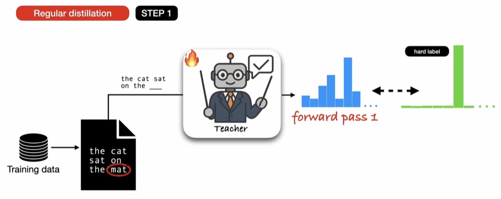
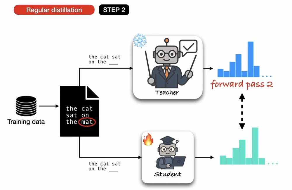
Meta says that codistillation from Llama 4 Behemoth during pre-training amortized the expensive teacher forward passes needed to compute distillation targets for most of Llama 4 Maverick’s training data.[5] The distinction becomes clearer by separating regular distillation into two phases.

Step 1: train the teacher. A forward pass through the teacher produces a distribution that is compared with the hard label, and the resulting loss updates the teacher.

Step one of regular distillation. A trainable teacher receives an incomplete sentence, produces a vocabulary distribution, compares it with the one-hot hard label for mat, and updates its weights. — Regular distillation begins by training the teacher against the hard target. Source: Julia Turc, “Knowledge Distillation: How LLMs train each other” [8].

Step 2: train the student. After the teacher has been trained and frozen, another forward pass through it produces the soft label used to train the student.

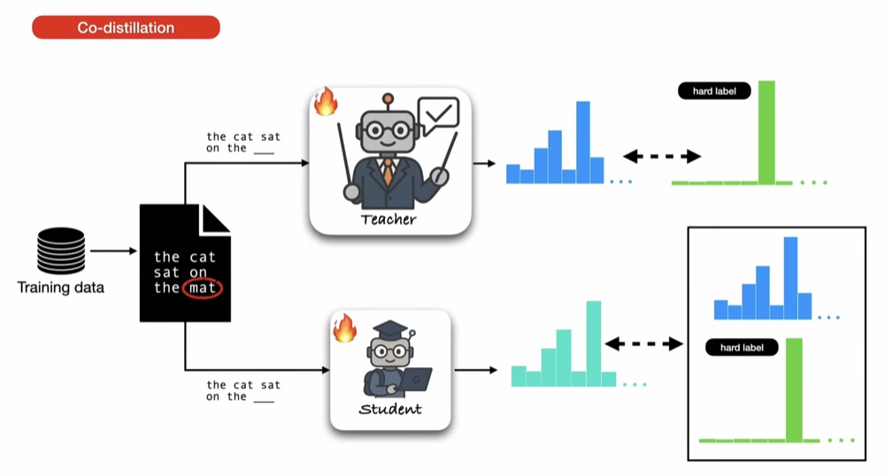
Step two of regular distillation. A frozen teacher and a trainable student receive the same incomplete sentence, produce vocabulary distributions, and the student learns to match the teacher's output. — Student training requires a second teacher forward pass to generate the soft target. Source: Julia Turc, “Knowledge Distillation: How LLMs train each other” [8].

In the co-distillation scheme illustrated below, the teacher and student are trained at the same time. The teacher’s forward pass serves two purposes: its prediction is compared with the hard target to update the teacher, and the same prediction immediately becomes a soft target for the student. The teacher therefore does not need to be rerun later over the same data solely to generate distillation targets.[8]

The tradeoff is that the teacher is still learning, so its early soft targets may be inaccurate. Meta’s loss dynamically weights soft and hard targets, allowing the hard labels to keep the student grounded while the teacher improves.[5]

Codistillation pipeline in which a trainable teacher and trainable student process the same incomplete sentence simultaneously. The teacher learns from the one-hot hard label, while its current vocabulary distribution also supplies a soft target for the student. — Codistillation reuses the teacher's current forward pass to train both the teacher and student together. Source: Julia Turc, “Knowledge Distillation: How LLMs train each other” [8].

Black-box distillation

Adapted from Sergei Parfenov, “How Model Distillation Actually Works (and What the ‘China Distilled Our Model’ Headlines Really Mean)”.

Headlines regularly claim that one AI lab distilled a model developed by another lab. Most of the methods discussed above assume access to the teacher’s logits or complete output distribution. This is white-box distillation, and it requires access to the model’s internals or full probability outputs.

A closed commercial API for a model such as Claude or GPT does not expose the raw logits or full vocabulary distribution needed for white-box distillation. It primarily exposes generated text. This forces a black-box distillation approach, where the student learns from the teacher’s text outputs without access to its parameters or logits.[13]

The standard black-box recipe is the sequence-level distillation or behavioral-cloning setup described earlier:

Prompt the teacher with a large and diverse collection of inputs.
Collect the teacher’s generated answers.
Build a synthetic dataset of (prompt, teacher answer) pairs.
Fine-tune the student on that dataset with supervised fine-tuning, optionally followed by preference optimization or reinforcement learning.

Because the student observes only sampled text, it loses the dark knowledge contained in the teacher’s soft labels. Even so, a large, high-quality synthetic dataset from a strong teacher can transfer a remarkable amount of capability.

This also explains why claims that model X learned from model Y’s outputs are difficult to prove. Black-box distillation does not require copying a weights file. The observable evidence is indirect: shared stylistic quirks, self-identification mistakes, or other statistical fingerprints in behavior. Such fingerprints can reveal similarity between model outputs, but they do not by themselves establish the provenance of the training data.[14]

Distillation scaling laws

A distillation scaling law predicts student performance from three main factors:[10]

Student model size. A larger student has more capacity to learn from the teacher.
Distillation tokens. More training tokens give the student more opportunities to learn from the teacher signal.
Teacher quality. The teacher’s validation loss summarizes the effect of its size and training data on the signal supplied to the student.

These relationships follow a power law, making improvements predictable but subject to diminishing returns. The best teacher depends on the student: a small student can use a weaker teacher to save compute, while a larger student generally needs a stronger teacher signal to realize further gains.[10]

A stronger teacher does not always produce a better student. If the gap between their learning capacities is too large, the student may struggle to imitate the teacher and can perform worse than it would with a somewhat weaker teacher. This is called the capacity gap.[10]

A student can also sometimes outperform its teacher. When a stronger pretrained student learns from a weaker supervisor and then exceeds that supervisor’s performance, the phenomenon is called weak-to-strong generalization.[11]

On-Policy Distillation

Adapted from Zachary Huang, “On-Policy Distillation in 20 Min” and Thinking Machines Lab, “On-Policy Distillation”.

Motivation

In the comparison below, off-policy distillation⁵ is standard supervised fine-tuning on teacher-generated solutions. The teacher writes a solution, and the student trains on that fixed text. This is relatively cheap, but it creates a distribution mismatch: the student learns from trajectories generated by the teacher during training, then must condition on its own earlier tokens at inference time. It never trains directly on the mistakes it makes when generating independently, so performance can plateau.[15]

Reinforcement learning fixes the mismatch by letting the current student generate its own attempts and then grading them. In outcome-based RL, however, a long sampled response may receive only one sparse reward at the end. The method can improve benchmark performance, but it spends substantial sampling and training compute to obtain that limited feedback.

On-policy distillation keeps the part of RL that works, namely learning from the student’s own attempts, while making the feedback dense. The student generates a trajectory, and the teacher supplies a next-token distribution at every prefix of that student-written trajectory. The student therefore receives a training signal at every token rather than only a final outcome reward.

Title page and abstract of the Qwen3 Technical Report, which describes using knowledge from flagship models to train competitive smaller models with less compute. — The Qwen3 Technical Report presents strong-to-weak distillation as a way to reduce the cost of training smaller models. Source: Qwen Team [16].

Qwen3-8B benchmark table comparing off-policy distillation, reinforcement learning, and on-policy distillation. On-policy distillation has the highest scores and lists 1,800 GPU-hours compared with 17,920 for reinforcement learning. — On Qwen3-8B, on-policy distillation achieved the strongest result in every reported benchmark column while listing 1,800 GPU-hours, compared with 17,920 for reinforcement learning. Source: Qwen Team [16], Table 21.

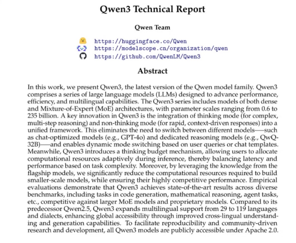
The Qwen3 comparison makes the compute tradeoff concrete. On-policy distillation produced the highest score in all six reported benchmark columns, using about one tenth of the GPU-hours listed for reinforcement learning: 1,800 instead of 17,920.[16]

The underlying problem was identified clearly by Rishabh Agarwal and colleagues in 2023. A student trained only on fixed outputs can drift as soon as it generates its own response, because each imperfect token changes the context for the tokens that follow. Their Generalized Knowledge Distillation method instead lets the student produce its own sequences and asks the teacher to provide token-level feedback on those sequences. In short, the student writes, and the teacher grades every token.[15]

The 2025 Thinking Machines post helped popularize the technique through a practical internal-assistant case study. The goal was to teach a model knowledge from a company’s private documents without sacrificing its existing ability to follow instructions.

In their experiments, continuing training on the internal documents during mid-training successfully taught the domain knowledge. It also caused catastrophic forgetting: as the network absorbed the new data, some of its post-trained assistant behavior was overwritten. In the reported experiment, Qwen3-8B’s internal-QA score rose from 18% to 43% after document-only mid-training, while its instruction-following score fell from 85% to 45%.[17]

The researchers then mid-trained on a 70:30 mix of internal documents and chat data and applied on-policy distillation, using the earlier Qwen3-8B checkpoint as the teacher. Distillation raised internal QA from 36% to 41% and nearly restored instruction following from 79% to 83%, close to the original 85%. The model retained the new domain knowledge while recovering almost all of its assistant behavior.[17]

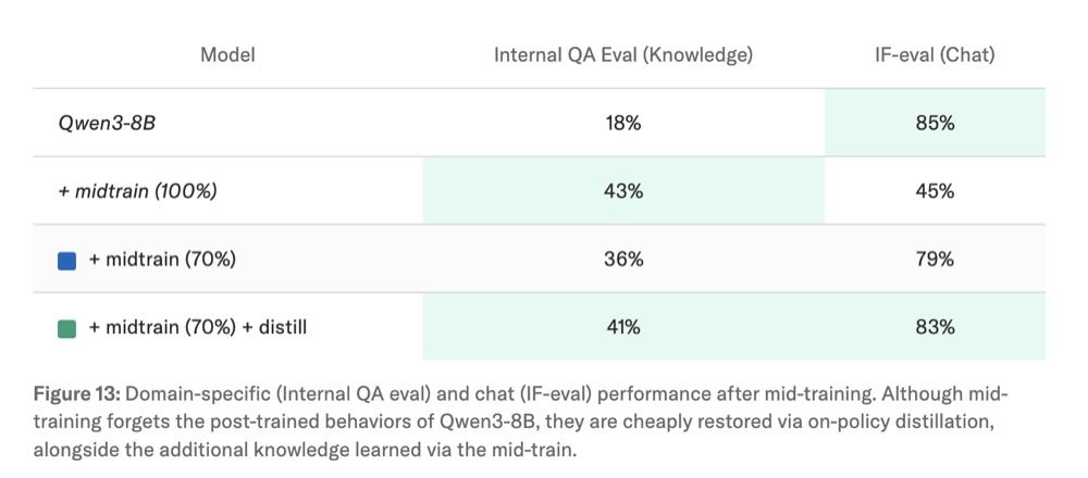
Table comparing Qwen3-8B before and after internal-document mid-training and on-policy distillation. A 70 percent mid-training mix followed by distillation reaches 41 percent on internal QA and 83 percent on instruction following. — On-policy distillation recovered nearly all instruction-following performance while preserving the knowledge learned during mid-training. Source: Thinking Machines Lab [17], Figure 13.

The takeaway is that, in these examples, on-policy distillation costs about one tenth as much as reinforcement learning and can even repair catastrophic forgetting.[16][17]

A distributional account of the same effect argues that the on-policy data is what protects existing capabilities. Because the student samples its own responses, training pressure stays in the region of the distribution the model already visits, rather than dragging it toward an arbitrary external target the way supervised fine-tuning does. In that analysis, on-policy distillation students forgot less than the supervised teacher they were distilled from, even when that teacher was itself already degraded.[26]

How it works

Suppose we are training a model to solve the arithmetic prompt 2 + 3 × 4 = ?. The correct answer is $14$ because multiplication comes before addition: $3\times4=12$ , then $2+12=14$ . A model can instead make the tempting mistake of adding first, obtaining $5\times4=20$ .

SFT, RL, and on-policy distillation differ in who writes the training trajectory and how that trajectory is graded:

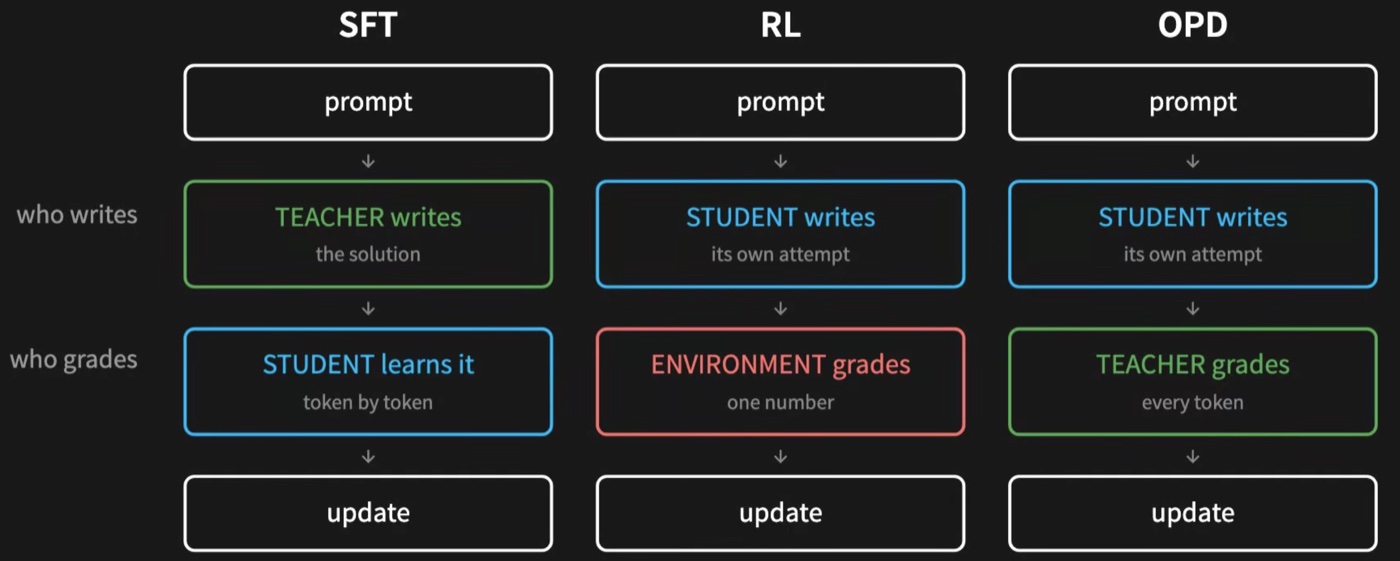
Three training pipelines compare supervised fine-tuning, reinforcement learning, and on-policy distillation. In SFT the teacher writes and the student learns token by token. In RL the student writes and the environment returns one score. In OPD the student writes and the teacher grades every token. — SFT is off-policy with dense token supervision, RL is on-policy with a sparse outcome reward, and on-policy distillation is on-policy with dense teacher feedback. Source: Zachary Huang [18].

Supervised fine-tuning. The teacher might provide the worked solution 3 × 4 = 12, then 2 + 12 = 14. The student learns to reproduce this clean teacher-written text token by token. It never trains on a prefix containing its own arithmetic mistake, so it has not learned how to recover when that mistake appears at inference time.

Reinforcement learning. The student writes its own attempts, and an environment checks each final answer. For example:

Student attempt	Final answer	Reward
`2 + 3 = 5, then 5 × 4 = 20`	$20\neq14$	$0$
`3 × 4 = 12, then 2 + 12 = 14`	$14=14$	$1$

This feedback trains on the student’s own behavior, but the verifier returns only one number for the entire attempt. A reward of $0$ reveals that the first solution failed without identifying which step introduced the error.

On-policy distillation. The student generates the same attempted solution, but the teacher evaluates it token by token.

The per-token grade can be based on reverse KL divergence. Reusing the earlier notation, let $q_\theta$ be the student distribution, $p_T$ the fixed teacher distribution, and $h_t$ the prompt plus all tokens before position $t$ . The reverse KL at that prefix is

D_{\mathrm{KL}}\!\left( q_\theta(\cdot\mid h_t)\parallel p_T(\cdot\mid h_t) \right) = \mathbb{E}_{x\sim q_\theta(\cdot\mid h_t)} \!\left[ \log q_\theta(x\mid h_t)-\log p_T(x\mid h_t) \right].

The student distribution appears first, so the expectation is over the student’s own possible next tokens. This is the on-policy part. For a token $x_t$ actually sampled by the student, the log-ratio

\widehat d_t = \log q_\theta(x_t\mid h_t) - \log p_T(x_t\mid h_t)

is a one-sample estimate of that per-prefix reverse KL. An RL-style update can use $A_t=-\widehat d_t$ as a per-token advantage, giving lower advantage to tokens the student considers much more likely than the teacher does.[17]

Unlike RL, where the environment penalizes the student only for the wrong answer at the end, on-policy distillation can identify the token where the trajectory first goes wrong. Here = 5 is that token, so it receives a large reverse-KL penalty of about $3.9$ . Once the student has sampled = 5, that mistake becomes part of the context. Conditioned on this new context, the teacher also considers the following green tokens plausible, so they receive much smaller reverse-KL penalties of about $0.1$ . The teacher therefore concentrates the punishment on the earlier mistake instead of repeatedly blaming the final answer.[15][17]

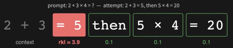
The incorrect attempt 2 plus 3 equals 5, then 5 times 4 equals 20. The first mistaken token, equals 5, has a reverse-KL penalty of 3.9, while each locally plausible continuation has a penalty of 0.1. — Dense feedback assigns the large penalty to the first token where the student's trajectory departs from the teacher. Later tokens can remain plausible after conditioning on that mistake. Source: Zachary Huang [18].

A 500-token rollout therefore gives standard RL one outcome-level training signal, while on-policy distillation can provide 500 token-level signals, one for each sampled token.

For the first wrong token, let $h_t=$ 2 + 3, and suppose the student assigns probability $0.90$ to = 5 while the teacher assigns it $0.02$ and instead assigns $0.88$ to × 4. If the student samples = 5, its log-ratio is

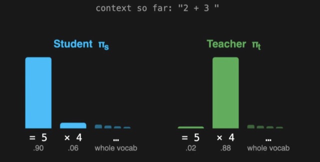
Student and teacher next-token probability distributions after the context 2 plus 3. The student assigns probability 0.90 to equals 5, while the teacher assigns probability 0.88 to times 4 and only 0.02 to equals 5. — At the same prefix, the student strongly favors the incorrect token `= 5`, while the teacher favors `× 4`. This distribution-level disagreement provides a dense training signal. Source: Zachary Huang [18].

\widehat d_t = \log(0.90)-\log(0.02) = \log(45) \approx 3.81\ \text{nats}.

This large positive value becomes an advantage of approximately $-3.81$ , strongly pushing the student away from that token in the same context. In contrast to a single reward of $0$ for the whole response, the signal identifies where the student’s probability distribution first diverged sharply from the teacher.

Toy rollout

Let the batch contain one rollout ( $B=1$ ), with four generated tokens ( $T=4$ ) and a vocabulary of eight tokens ( $V=8$ ). Before selection, each model produces a $[1,4,8]$ tensor containing a log-probability for every vocabulary item at every position. gather keeps only the log-probability of the token the student actually sampled, reducing each tensor to $[1,4]$ . The PyTorch-like sketch omits prompt concatenation and the causal shift for brevity.

Dry run for a batch of one four-token rollout. The student log-probabilities are minus 0.1, minus 0.2, minus 0.1, and minus 0.3. The teacher log-probabilities are minus 4.0, minus 0.3, minus 0.2, and minus 0.4, producing reverse-KL estimates of 3.9, 0.1, 0.1, and 0.1 and advantages of minus 3.9, minus 0.1, minus 0.1, and minus 0.1. — The code gathers both models' log-probabilities for the student's sampled tokens, then converts their differences into per-token advantages. The dry run shows the first wrong token receiving nearly all of the corrective signal. Source: Zachary Huang [18].

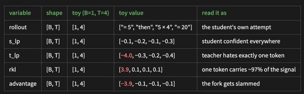
In the dry run, subtracting the teacher log-probabilities from the student’s gives $[3.9,0.1,0.1,0.1]$ . Negating those values produces the token-level advantages $[-3.9,-0.1,-0.1,-0.1]$ . Using the rounded values shown, the first token contributes $3.9/(3.9+0.1+0.1+0.1)\approx93\%$ of the total reverse-KL signal.

Why on-policy distillation works

The reason copying such a teacher can improve the student has a precise form. Let $u$ denote a complete output sequence, let $q_k(u)$ be the current student policy held fixed while the teacher is constructed, and let $R(u)$ be its reward. Consider the following KL-regularized policy-improvement objective over a candidate policy $p$ :

p_T^\star = \underset{p}{\operatorname{arg\,max}} \left\{ \beta\,\mathbb{E}_{u\sim p}[R(u)] - D_{\mathrm{KL}}\!\left(p\parallel q_k\right) \right\},

where $\beta>0$ controls the strength of reward relative to the KL penalty. This objective has the closed-form optimum

p_T^\star(u) = \frac{1}{Z_k}\,q_k(u)e^{\beta R(u)}, \qquad Z_k = \mathbb{E}_{u\sim q_k}\!\left[e^{\beta R(u)}\right].

The factor $e^{\beta R(u)}$ tilts the current student toward high-reward responses, while $q_k(u)$ keeps the resulting teacher close to behavior the student can already produce. Now freeze this reward-tilted teacher, set $p_T=p_T^\star$ , and train a new student policy $q$ by minimizing reverse KL. The loss decomposes as

\begin{aligned} D_{\mathrm{KL}}\!\left(q\parallel p_T\right) &= \mathbb{E}_{u\sim q} \left[ \log\frac{q(u)}{p_T(u)} \right] \\ &= D_{\mathrm{KL}}\!\left(q\parallel q_k\right) - \beta\,\mathbb{E}_{u\sim q}[R(u)] + \log Z_k. \end{aligned}

Because $q_k$ and $Z_k$ are fixed during this update, minimizing the distillation loss is equivalent to maximizing expected reward while penalizing movement away from the current policy. Distillation toward the ideal reward-tilted teacher is therefore exactly a KL-regularized RL update. Its token-level decomposition also supplies a learning signal at every prefix, making the update much denser than one scalar reward per trajectory.

A real teacher will not equal $p_T^\star$ exactly. The closer its distribution is to this reward tilt, the better distillation approximates a reward-improving step. If the teacher is not better on reward, or is too far from the student’s distribution to grade its rollouts reliably, that policy-improvement interpretation no longer holds. The practical requirement is therefore a teacher that is both better and close enough to copy.

Limitations

The logit-based form of on-policy distillation described here cannot be used directly when the teacher is available only through a black-box API that returns text but not token log-probabilities. Without those probabilities, the student cannot compute the per-token divergence. Specialized black-box distillation methods must replace the missing logit signal with another form of feedback.[13]

The direct per-token objective also assumes compatible tokenization. If the teacher and student use different tokenizers, one student token may correspond to several teacher tokens, so their vocabulary indices and token positions cannot be matched directly. TRL’s experimental GOLD Trainer works around this by aligning decoded text spans and merging the associated probabilities before computing the distillation loss.[23]

Distillation is fundamentally an imitation objective, so it should not be expected by itself to push the capability frontier beyond the best available teacher. A student can occasionally outperform its teacher, as in the weak-to-strong generalization phenomenon discussed above, but that is not guaranteed. When the goal is to discover behavior better than the strongest teacher can demonstrate, reinforcement learning with an external reward or verifier remains the standard tool.[11]

OPD being used in practice

On-policy distillation is becoming a standard post-training tool. DeepSeek-V4 trains domain-specific experts with SFT and GRPO, then consolidates their capabilities into one model through on-policy distillation.[24] Nemotron 3 Ultra similarly uses multi-teacher on-policy distillation to merge more than ten specialized teachers through dense token-level guidance on student-generated rollouts.[25] In a matched-architecture experiment, Thinking Machines recovered the performance of an RL-trained teacher in roughly 7–10 times fewer gradient steps and estimated a 50–100 times reduction in total compute.[17]

A useful teacher has two properties: it earns higher reward than the student, and it remains close enough for the student to imitate. One option is a larger model from the same family, which tends to share the student’s training distribution while being more capable. Another is a domain expert obtained by post-training a common base model with SFT or RL. Closeness matters because the teacher must still provide meaningful probabilities on prefixes generated by the student. Nemotron 3 Ultra, for example, reports that a large teacher-student distribution mismatch weakened supervision and used a short warmup stage to bring their distributions closer before distillation.[25]

On-Policy Self-Distillation

Adapted from Zhao et al., “Self-Distilled Reasoner” and Zachary Huang, “On-Policy Distillation in 20 Min”.

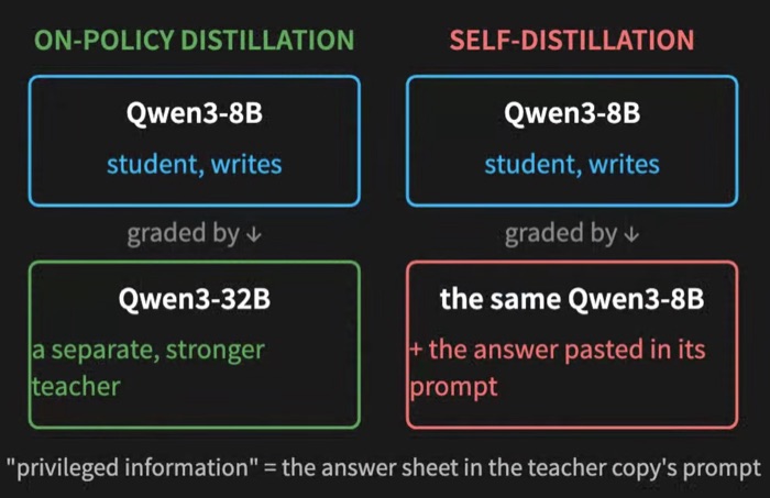
Three contemporaneous works, Self-Distilled Reasoner, Self-Distillation Enables Continual Learning, and Reinforcement Learning via Self-Distillation, converged on the same basic idea: why pay for a separate teacher if the model can grade itself under a more informative context? The same model is used twice. The student view sees the ordinary prompt, while the teacher view also receives privileged information such as a reference solution, an expert demonstration, or environment feedback.[19][20][21]

In ordinary OPD, a weaker student generates the rollout and a separate, stronger teacher grades every sampled token. On-policy self-distillation (OPSD) keeps the student-generated rollout but replaces the external teacher with another evaluation of the same model. For reasoning tasks, the privileged teacher prompt can include the verified reference answer. The teacher does not write a replacement solution; it scores the student’s exact trajectory while having access to that additional context.[19]

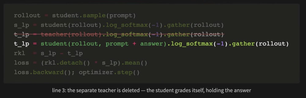
Comparison of on-policy distillation and on-policy self-distillation. In OPD, Qwen3-8B writes and a separate Qwen3-32B teacher grades it. In self-distillation, Qwen3-8B both writes and grades, with the reference answer added to the teacher copy's prompt. — OPD uses a separate, stronger teacher. OPSD uses the same model as both student and teacher, but gives the teacher view privileged information. Source: Zachary Huang [18].

Conceptually, the implementation changes one line. Instead of calling a separate teacher to score the rollout, the training loop calls the student again and adds the reference answer to its context. In an actual implementation, gradients through this teacher-side evaluation are stopped; only the ordinary student view is updated.[19]

PyTorch-like on-policy distillation code where the separate teacher scoring call is crossed out and replaced by a second call to the student conditioned on the prompt and reference answer. — The OPSD proposal replaces the external teacher call with a privileged evaluation of the same model. Source: Zachary Huang [18].

Competence versus privilege

This approach depends on a strong assumption: the privileged self-teacher must behave like a genuinely better policy, not merely like the same policy holding an answer sheet. Rishabh Tiwari argues that naive privileged self-distillation can fail in three related ways:[22]

Feedback leakage. Training can teach the student to write as though it always has access to a hint, reference solution, or earlier feedback. At inference time that context is absent, but the model may still refer to feedback or evidence it was never given.
Overconfidence. The model can become less likely to re-examine its reasoning because the privileged teacher was conditioned on the answer from the start.
Poorer out-of-distribution generalization. In the reported comparisons, the weakness becomes much clearer outside the training distribution, where naive self-distillation falls 6–25 points below RL across the evaluated settings.[22]

The arithmetic example makes the distinction concrete. A stronger OPD teacher can independently derive that 2 + 3 × 4 = 14; that is a competence advantage. A privileged copy of the student can simply read 14 from the reference answer and construct reasoning backward from it; that is only a contextual advantage. Seeing the destination can make rationalization easier, but it does not necessarily teach the unprivileged student how to find that destination at inference time.

Ground truth itself is not the problem. A verifier can safely use the correct answer to evaluate a solution the student generated independently. The risk comes from promoting an answer-conditioned copy of the student into a dense teacher and assuming that every distributional change caused by the answer is useful supervision.

Teacher advantage	Example	What is being transferred
Real capability	A stronger model solves a chemistry problem because it understands the chemistry better than the student.	Knowledge and reasoning the deployed student can learn to reproduce.
Privileged context only	The same student is shown the correct answer and asked to produce reasoning that leads to it.	A tendency to rationalize from information that will be unavailable at inference time.

Using an older checkpoint of the same model as the teacher is not inherently a problem. It can work when that checkpoint genuinely produces behavior the new model should learn without receiving special hints. The useful criterion is not whether teacher and student share a model family; it is whether the teacher possesses a real capability or knowledge advantage rather than merely being shown clues that reveal the desired answer.

To read

To watch

“On Policy Distillation - How the big AI labs actually train their LLMs”
“On-Policy Distillation in 20 Min”, Zachary Huang
“How On Policy Self Distillation Works”, Sasha Rush
“Knowledge Distillation: How LLMs train each other”, Julia Turc

Suppose a model assigns the logits $[2, 1, 0]$ to the classes cat, dog, and bird. Softmax exponentiates each logit and divides it by the sum of all three exponentiated logits:

Class	Logit $z_i$	Softmax probability $p_i$
Cat	$2$	$\frac{e^2}{e^2 + e^1 + e^0} = 0.665$
Dog	$1$	$\frac{e^1}{e^2 + e^1 + e^0} = 0.245$
Bird	$0$	$\frac{e^0}{e^2 + e^1 + e^0} = 0.090$

The probabilities sum to $0.665 + 0.245 + 0.090 = 1.000$ , and cat receives the highest probability. ↩

Consider a three-class example with teacher logits $v=(\log 9,0,0)$ , student logits $z=(\log 4,0,0)$ , temperature $T=2$ , and hard label $y=(1,0,0)$ . Let $\alpha=0.8$ and $\beta=0.2$ .

Component	Calculation	Value
Teacher soft targets	$p^{(2)}=\frac{(3,1,1)}{3+1+1}$	$(0.6000,0.2000,0.2000)$
Student soft output	$q^{(2)}=\frac{(2,1,1)}{2+1+1}$	$(0.5000,0.2500,0.2500)$
Student hard output	$q^{(1)}=\frac{(4,1,1)}{4+1+1}$	$(0.6667,0.1667,0.1667)$
Soft loss	$-[0.6\log(0.5)+0.2\log(0.25)+0.2\log(0.25)]$	$0.9704$
Hard loss	$-[1\log(0.6667)+0\log(0.1667)+0\log(0.1667)]$	$0.4055$
Combined loss	$0.8(2^2)(0.9704)+0.2(0.4055)$	$3.1864$

The soft branch trains the student to match the teacher’s complete distribution, while the hard branch rewards probability assigned to the correct first class. The factor $T^2$ rescales the soft-loss contribution; it does not alter the probabilities themselves. ↩

Suppose the static distillation corpus contains the prompt “Choose two colors:” and the teacher-produced output $u=(\text{red},\text{blue})$ . For a toy vocabulary $\mathcal{V}=\{\text{red},\text{blue},\text{green}\}$ , consider these teacher and student distributions:

Position and context	Teacher $p$ over (red, blue, green)	Student $q$ over (red, blue, green)	Per-token cross-entropy
$j=1$ : “Choose two colors:”	$(0.70,0.20,0.10)$	$(0.60,0.25,0.15)$	$-[0.70\log(0.60)+0.20\log(0.25)+0.10\log(0.15)]=0.825$
$j=2$ : “Choose two colors: red”	$(0.10,0.80,0.10)$	$(0.20,0.65,0.15)$	$-[0.10\log(0.20)+0.80\log(0.65)+0.10\log(0.15)]=0.695$

Using natural logarithms, the sequence loss is $\mathcal{L}_{\text{token-KD}}=0.825+0.695=1.520$ . Although the teacher selected “red” and then “blue,” every vocabulary probability contributes to the loss at each position. ↩

Suppose the prompt is “Translate Guten Morgen into English.” Each complete-sequence probability is the product of the teacher’s conditional token probabilities. For a coherent toy distribution:

Candidate sequence or probability mass	Autoregressive factorization and calculation
“Good morning.”	$p(\text{Good}\mid s)\,p(\text{morning}\mid s,\text{Good})\,p(\text{.}\mid s,\text{Good morning})=0.85\times0.86\times0.85=0.62135\approx0.62$
“Morning.”	$p(\text{Morning}\mid s)\,p(\text{.}\mid s,\text{Morning})=0.10\times0.80=0.080$
“Have a good morning.”	$p(\text{Have}\mid s)\,p(\text{a}\mid s,\text{Have})\,p(\text{good}\mid s,\text{Have a})\,p(\text{morning}\mid s,\text{Have a good})\,p(\text{.}\mid s,\text{Have a good morning})=0.04\times0.90^4=0.026244\approx0.026$
All remaining sequences combined	$1-(0.62135+0.080+0.026244)=0.272406\approx0.273$

Beam search selects $\hat{u}=$ “Good morning.” Sequence-level KD replaces the teacher’s full sequence distribution with a point mass on this one output. Suppose the student assigns the following conditional probabilities to its three tokens:

Position	Student prediction	Student probability	Token loss
$1$	$q(\text{Good}\mid s)$	$0.70$	$-\log(0.70)=0.357$
$2$	$q(\text{morning}\mid s,\text{Good})$	$0.80$	$-\log(0.80)=0.223$
$3$	$q(\text{.}\mid s,\text{Good morning})$	$0.90$	$-\log(0.90)=0.105$

The student’s probability for the complete sequence is $q(\hat{u}\mid s)=0.70\times0.80\times0.90=0.504$ . Therefore, $\mathcal{L}_{\text{seq-KD}}=-\log(0.504)=0.357+0.223+0.105=0.685$ . The other teacher candidates do not contribute after the point-mass approximation. ↩

Off-policy means the student learns from data or target outputs generated by a policy or source different from the policy currently being trained. Offline means training happens without interacting with the environment during training, using a fixed dataset. ↩

Bibliography

Jianping Gou, Baosheng Yu, Stephen J. Maybank, and Dacheng Tao, “Knowledge Distillation: A Survey,” International Journal of Computer Vision, vol. 129, pp. 1789–1819, 2021.
Hopsworks, “LLM Temperature,” MLOps Dictionary, 2026.
Geoffrey Hinton, Oriol Vinyals, and Jeff Dean, “Distilling the Knowledge in a Neural Network,” arXiv preprint arXiv:1503.02531, 2015.
Yoon Kim and Alexander M. Rush, “Sequence-Level Knowledge Distillation,” Proceedings of the 2016 Conference on Empirical Methods in Natural Language Processing, pp. 1317–1327, 2016.
Meta AI, “The Llama 4 herd: The beginning of a new era of natively multimodal AI innovation,” Meta AI Blog, 2025.
DeepSeek-AI et al., “DeepSeek-R1: Incentivizing Reasoning Capability in LLMs via Reinforcement Learning,” arXiv preprint arXiv:2501.12948, 2025.
Google for Developers, “Introducing Gemma 3: The Developer Guide,” Google Developers Blog, 2025.
Julia Turc, “Knowledge Distillation: How LLMs train each other,” YouTube, 2025.
Gemma Team, Google DeepMind, “Gemma 3 Technical Report,” arXiv preprint arXiv:2503.19786, 2025.
Dan Busbridge, Amitis Shidani, Floris Weers, Jason Ramapuram, Etai Littwin, and Russ Webb, “Distillation Scaling Laws,” Proceedings of the 42nd International Conference on Machine Learning, 2025.
Collin Burns et al., “Weak-to-Strong Generalization: Eliciting Strong Capabilities With Weak Supervision,” arXiv preprint arXiv:2312.09390, 2023.
Geoffrey Hinton, “Dark Knowledge,” TTIC Distinguished Lecture Series, 2014.
Tianzhu Ye, Li Dong, Zewen Chi, Xun Wu, Shaohan Huang, and Furu Wei, “Black-Box On-Policy Distillation of Large Language Models,” arXiv preprint arXiv:2511.10643, 2025.
Teppei Suzuki, Ryokan Ri, and Sho Takase, “Natural Fingerprints of Large Language Models,” arXiv preprint arXiv:2504.14871, 2025.
Rishabh Agarwal, Nino Vieillard, Yongchao Zhou, Piotr Stanczyk, Sabela Ramos, Matthieu Geist, and Olivier Bachem, “On-Policy Distillation of Language Models: Learning from Self-Generated Mistakes,” arXiv preprint arXiv:2306.13649, 2023.
Qwen Team, “Qwen3 Technical Report,” arXiv preprint arXiv:2505.09388, 2025.
Kevin Lu and Thinking Machines Lab, “On-Policy Distillation,” Thinking Machines Lab, 2025.
Zachary Huang, “On-Policy Distillation in 20 Min,” YouTube, 2026.
Siyan Zhao, Zhihui Xie, Mengchen Liu, Jing Huang, Guan Pang, Feiyu Chen, and Aditya Grover, “Self-Distilled Reasoner: On-Policy Self-Distillation for Large Language Models,” arXiv preprint arXiv:2601.18734, 2026.
Idan Shenfeld, Mehul Damani, Jonas Hübotter, and Pulkit Agrawal, “Self-Distillation Enables Continual Learning,” arXiv preprint arXiv:2601.19897, 2026.
Jonas Hübotter, Frederike Lübeck, Lejs Behric, Anton Baumann, Marco Bagatella, Daniel Marta, Ido Hakimi, Idan Shenfeld, Thomas Kleine Buening, Carlos Guestrin, and Andreas Krause, “Reinforcement Learning via Self-Distillation,” arXiv preprint arXiv:2601.20802, 2026.
Rishabh Tiwari, “Why On-Policy Distillation Works and Naive Self-Distillation Doesn't,” X, 2026.
Hugging Face, “General Online Logit Distillation (GOLD) Trainer,” TRL documentation, 2026.
DeepSeek-AI, “DeepSeek-V4: Towards Highly Efficient Million-Token Context Intelligence,” Hugging Face model card, 2026.
NVIDIA, “Nemotron 3 Ultra: Open, Efficient Mixture-of-Experts Hybrid Mamba-Transformer Model for Agentic Reasoning,” Technical report, 2026.
nrehiew, “SFT, RL, and On-Policy Distillation Through a Distributional Lens,” nrehiew.github.io, 2026.