← All notes

Efficient Reinforcement Learning for LLMs

July 29, 2026 · Updated July 31, 2026

Synchronous RL

Every GPU starts the iteration holding the same policy, $\pi_t$. Each row in the animation is one GPU generating responses, and no two rollouts are the same length, because language model outputs aren’t the same length:

So some GPUs finish quickly while others keep generating. That wouldn’t matter if each GPU could move on alone, but synchronous RL runs one strict sequence per iteration:

Training consumes the entire batch, so if even one worker hasn’t finished, the batch is incomplete and everyone waits. Step times are therefore dictated by whatever sample takes the longest to complete, not by the average one. Only once the slowest GPU is done does every GPU switch from inference to training, and the model advances:

π_t
 │
 │  Gradient updates (PPO/GRPO/etc.)
 ▼
π_{t+1}

One iteration, concretely

Suppose you have 8 GPUs, all holding the current policy $\pi_t$. Each one generates many complete responses:

GPU 1: 100 prompts → 100 responses
GPU 2: 100 prompts → 100 responses
...
GPU 8: 100 prompts → 100 responses

Those 800 rollouts are what the rewards, advantages, and PPO loss are computed from. Then comes not one gradient step but several, often multiple epochs over the same collected data, with $\pi_t$ held fixed in the denominator of every importance ratio:

Collect rollouts using π_t
      │
      ├── Store actions
      ├── Store rewards
      ├── Store old log-probabilities
      │
      ▼
Epoch 1:  ratio = π_θ / π_t
      ▼
Epoch 2:  ratio = π_θ / π_t
      ▼
Epoch 3:  ratio = π_θ / π_t
      ▼
Epoch 4:  ratio = π_θ / π_t
      ▼
Done
      ▼
Rename current policy as π_{t+1}

Only after those optimization steps finish do you have $\pi_{t+1}$, and only then can the next batch be collected with the updated model.

The animation simplifies this to make the synchronization visible: rather than hundreds of responses per GPU, it draws generate one rollout → wait → train → generate the next. The real loop is generate 100 rollouts → wait until every GPU finishes → train for several epochs → generate the next 100. The constraint it illustrates is the real one either way: training can’t start until all GPUs have finished collecting the current batch.

This is the naive version because it wastes the hardware. Toward the end of the generation phase, the GPU that drew the longest rollout is still decoding while the other seven sit idle, and again during training nobody generates.

That waste is visible in a throughput chart. Throughput here is generation throughput: how many tokens per second the fleet is decoding, summed across GPUs (one colored band per GPU in the chart below). It’s a direct read on how much of the hardware is actually doing work, since a GPU that has finished its rollouts and is waiting contributes nothing to the total.

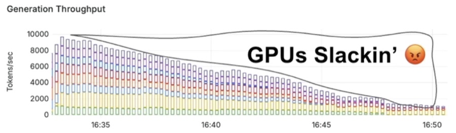
At the start, when every sampling request has just been launched, the GPUs are doing a lot of work and throughput peaks near 10,000 tokens/sec. It then decays for the rest of the phase, ending around 1,000: as requests finish, fewer and fewer GPUs still have anything to decode, and the fleet spends the tail of the phase waiting on the last few samples. The whole shaded region above the curve is throughput that was paid for and never used, which is why synchronous RL is a poor way to use these GPUs.

Everything that follows in this note is about removing that idle time.

Async Pipeline RL

To break the bottleneck, you have to break the condition that causes it: that training and sampling happen one after the other. Allowing training to run while sampling is still going is what makes an algorithm asynchronous. There are many ways to arrange that; the one discussed here is Pipeline RL.

Instead of every GPU doing everything, the fleet is split into two groups:

Sampling GPUs      Training GPUs

GPU 1              GPU 7
GPU 2              GPU 8
GPU 3
GPU 4
GPU 5
GPU 6

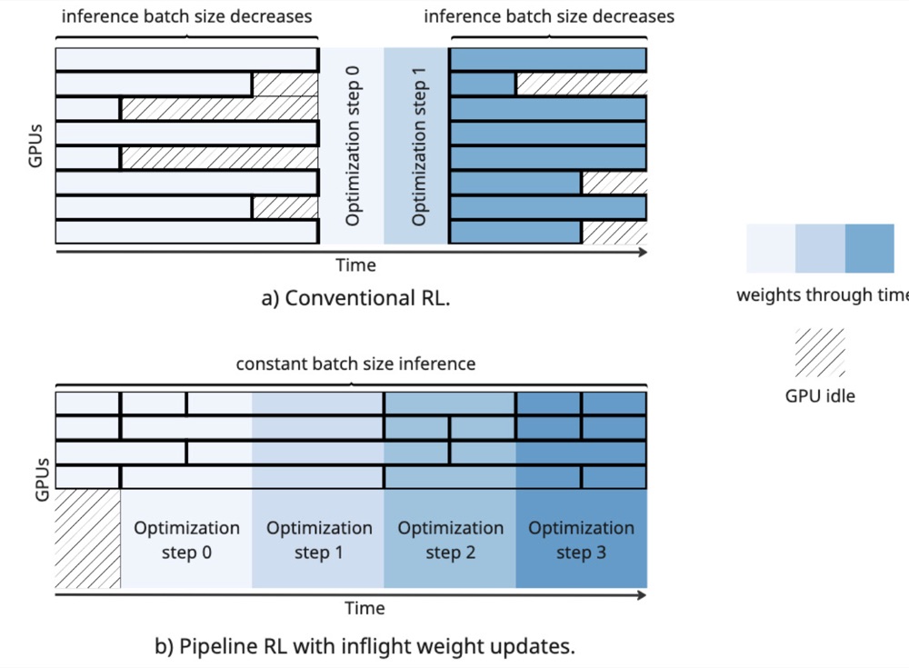
The sampling workers never stop; they run inference continuously at high batch size. As samples complete, they’re added to a queue, and the training workers pull a batch off that queue to train on. Once a batch has been trained on, the training workers propagate the new weights to every sampling worker. This is the part that really distinguishes Pipeline RL: a sampling worker might be in the middle of a sample, and its weights get updated anyway. That’s an in-flight weight update.

So the timeline no longer has phases. $\pi_t$ starts generating; while it generates, the learner trains $\pi_t \to \pi_{t+1}$; the moment training finishes, the new weights go straight to the samplers, and the next tokens come from $\pi_{t+1}$. Then $\pi_{t+2}$, and so on. The learner GPUs are always training and never wait for the samplers to finish.

The consequence is that a single sample can have several policy versions contributing to it. Put another way, some of the tokens in these samples are stale.

Why one rollout changes color partway through

Consider a model answering a single prompt:

That’s why a rollout boundary (a black box in the animation above) contains more than one color. One black box is one complete response, and unlike synchronous RL, that response may have been produced by several policies rather than one fixed one:

Token 1  (π_10)
Token 2  (π_10)
Token 3  (π_10)
--- training finishes ---
Token 4  (π_11)
Token 5  (π_11)
--- training finishes ---
Token 6  (π_12)
Token 7  (π_12)

PPO normally assumes one rollout maps to one policy. Pipeline RL breaks that: one rollout maps to many policy versions.

The importance ratio needs a per-token denominator

Standard PPO assumes every token in a rollout came from the same behavior policy, which is exactly what makes its importance ratio well defined: the behavior policy is just $\pi_t$, so

One optimizer step per batch

Pipeline RL isn’t doing the standard PPO-style multiple optimization epochs over a batch. Its loop is:

Collect some fresh data
        ↓
One optimizer step
        ↓
Immediately publish weights
        ↓
Collect more fresh data
        ↓
One optimizer step

There is almost no data reuse. One optimizer step per batch means every update is performed on nearly on-policy data, which is the whole point of publishing weights the instant a step completes.